Notice the advantages of ROS and the advantages of using a modular design. In the future, if we want a new path planner, the only code we need to adjust is the path planner node. This same logic holds for both the maps and controllers. Using ROS is not the only way to achieve this; for example, code with well-designed interfaces might accomplish the same thing. However, with ROS you benefit from a whole community designing and optimizing similar nodes that you can reuse.
Mapping and Plans
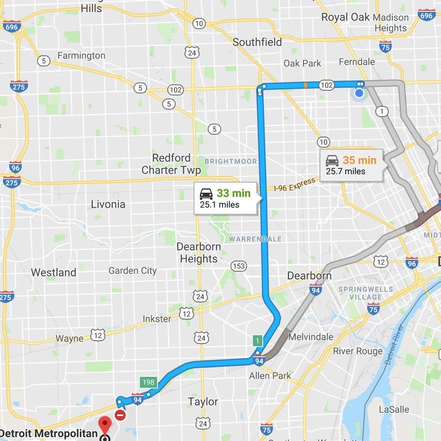
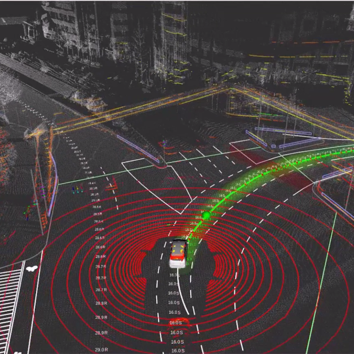
Mobile robots’ ability to move in an environment to satisfy a goal relies on some form of localization and planning, often with the help of maps. There is a significant body of work on different map representations and motion planning algorithms, exploiting tradeoffs such as their fidelity versus their cost versus their ability to capture unexpected events. For instance, the Husky robot (from Clearpath Robotics) builds a grid map as it moves and senses an unknown environment using the gmapping ROS package. On the other hand, self-driving cars usually provide navigation support by using predefined route maps, such as Google Maps, to identify viable trajectories. Autoware, an open-source self-driving stack, provides a hybrid model that combines static maps with sensor-built maps.
In this lab, we will instantiate just one kind of map and navigation algorithm to support our drone in flying to a goal without hitting any obstacles.
Clearpath Robotics
Google Maps
Autoware
Learning Objectives
At the end of this lab, you should understand:
- How to set up and interpret maps in ROS
- How to create and manage an occupancy grid map
- How to navigate a robot through the world to reach a goal with common motion planning algorithms
Lab Requirements
Retrieve the new code base for Lab 7 by running git pull.
Lab Overview
In this lab, we are going to get our drone to navigate through the world. We will need a map to represent the world and a path planner to generate a path that takes our drone to a target goal. The path planner will also need to make sure the path it creates is collision-free and safe for the drone to fly. To create collision-free safe paths, our drone path planner needs to know where the obstacles in the world are. If these obstacles are static and well known, a good way to represent them is by using maps.
To start, we will need a way to describe maps. By describing maps independently of any system, we will be able to reuse maps for different systems and change maps to expose our system to different worlds under simulation to validate its performance.
From a design perspective, it makes sense to allocate map handling functionality to its own node. That way, if multiple nodes are using the map and the incoming format of the maps changes, only this node is affected. This node should then consume a map in a specified format and make it available to other nodes as a standardized data structure containing a map.
Once a map is available, we will need an additional node to consume the map data structure and find a path to go from a starting location to a goal location. This node can send commands to the drone’s controllers (just like we did in the past labs). More specifically, our path planner node will transform the map into a graph which can then be searched using any standard graph searching algorithm. The path planner node will publish both a path as well as a waypoint. The path contains a list of waypoints consumed by the visualizer node to see the drone’s planned path. The path planner also publishes the next waypoint in the path to the geofence_and_mission node, which will move the drone to that waypoint (if it’s inside the geofence bounds).
Starting Code Base
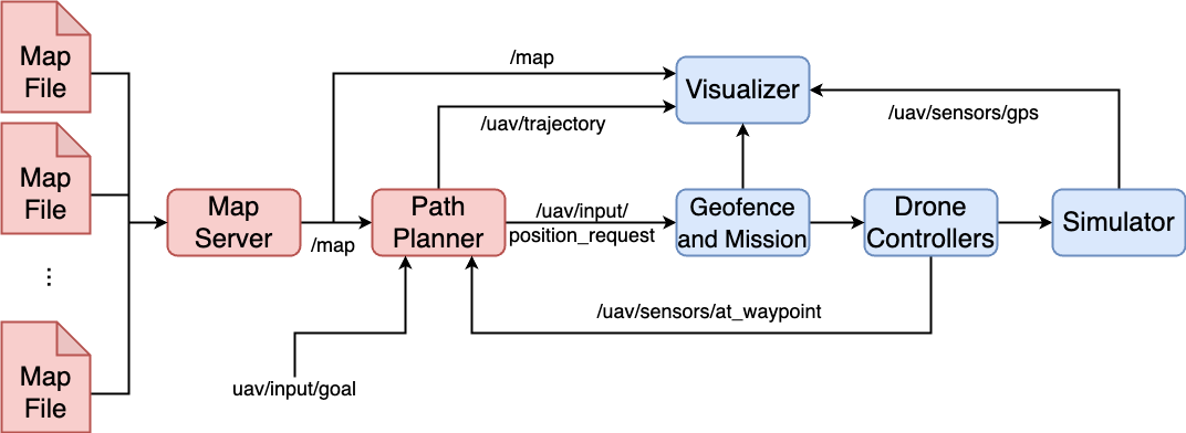
Let’s start to design our system and connect it to the existing system. We know we want to read maps from map files. A map message can then be published on the /map topic for our path planner to read. The path planner will compute a path to reach a goal (given on the topic /uav/input/goal). The path planner will publish the computed path on the topic /uav/path, as well as the next waypoint in the path on the topic /uav/input/position_request. The geofence_and_mission node subscribes to the position_request topic and, if the position is inside the geofence, sends messages to the drone’s controller requesting the next position. This is all shown below in the overview (red means unimplemented and blue means implemented and available for use):
Let’s see how it links into our existing system. After launching the simulator, run RQT graph. You will see the following graph (Note: Uncheck “Leaf topics” and “Dead Sinks”. Also change the dropdown to display “Nodes/Topics (All)”):
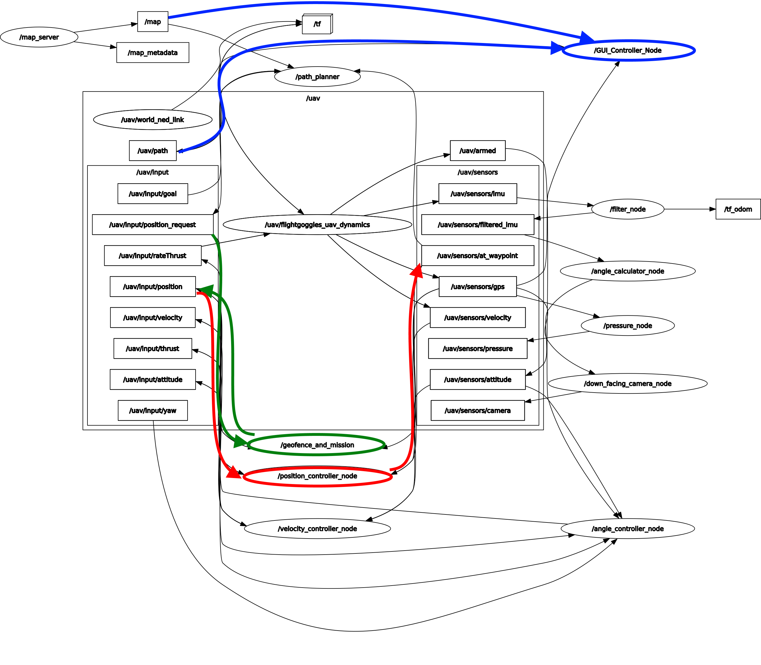
We first notice that neither the map server nor the path planner nodes have been implemented. We will need to do that in this lab. We can see that the GUI_Controller_Node, as well as the geofence_and_mission node, already exist. Let’s identify what topics they use and how they work.
-
(Green) We previously implemented the
geofence_and_missionnode, and used it to validate the waypoints send to the drone controllers. If you hover your mouse over this node, you will see that it publishes to the/uav/input/positiontopic. We also see that it subscribes touav/input/position_request. Thus, our path planner node will need to send position commands on the topic/uav/input/position_requestto control our drone and allow it to follow a path. -
(Red) Next, hover your mouse over the
position_controller_node. This node publishes to the topic/uav/sensors/at_waypoint. Other nodes can use this to determine if the drone is at the requested position or not. -
(Blue) Finally, take notice that the
GUI_Controller_Nodenow subscribes to two new topics/uav/pathand/map. Nothing publishes to these topics yet, and in this lab we will need to correct that. We will need for the path planner node to publish to the/uav/pathtopic and for our map node to publish to the/maptopic.
The Map Server
Let’s start by implementing the map server node. You might remember from previous labs that many of the nodes that perform common robotic tasks are readily available for download from the ROS community. Mapping is one of those common tasks that has been shared and packaged extensively. One of these available nodes is the map_server node. A quick search for ROS map server will result in the following webpage: https://wiki.ros.org/map_server
Reading the first line from this wiki we see that this node is what we need: “the map_server ROS Node, which offers map data as a ROS Service”. If we read through the wiki page, we will pick out a few main important points:
- Maps are stored as a pair of files (i.e. each map requires two files).
- The first file is a YAML file that describes the map meta-data.
- The second file contains the map data as an image file.
- The image file encodes the occupancy data.
Setting up the Map Server
The first thing we need to do is make the map_server node available to our project. To do that we can install the pre-compiled version of the map_server by running the command:
$ sudo apt-get install ros-melodic-map-server -y
The next thing we will need is a map file to check that the downloaded node works as expected. We will use one of the map files provided in our simulator. Let’s start a roscore and check that we are now able to launch the map_server node. To do that open three terminals and run the following commands:
Terminal 1: (remember roslaunch files automatically start a roscore. However we do not have a launch file yet, hence why we need to do this manually):
$ roscore
Terminal 2:
$ rosrun map_server map_server ~/CS4501-Labs/lab7_ws/src/flightcontroller/maps/map_medium0.yaml
>>> [ INFO] [1584732125.415783128]: Loading map from image "/.../src/flightcontroller/maps/map_medium0.png"
>>> [ INFO] [1584732125.416015567]: Read a 20 X 20 map @ 1.000 m/cell
We will learn more about this metadata later in the lab.
Terminal 3:
$ rostopic list
>>> /map
>>> /map_metadata
>>> ...
Finally, let’s look at what the /map topic contains. Echo the topic using:
Terminal 3:
$ rostopic echo /map
>>> header:
>>> ...
>>> info:
>>> ...
>>> data: [0, 0, 0, ..., 100, ..., 0]
You should see the meta data, the origin and then the raw data. To understand how maps are encoded, we first need to review occupancy grids.
Be sure to stop all of the above terminals before running the later portions of the lab.
Occupancy Grids
An occupancy grid is a probabilistic grid map, where each cell in the map is the probability that an obstacle is in that cell. When a map is known in advance and the obstacles are static, those probabilities tend to be either zero or one. When the maps are not known in advance but rather discovered by the robot, cells for which the sensors frequently detect obstacles (and cells that were never sensed) will end up with a higher probability of having an obstacle, and our robot will try to avoid them. Cells where obstacles are detected rarely and irregularly (likely due to sensor noise), will have a lower probability of having an obstacle, and our robot can assume that an obstacle does not occupy the cell. In the plot below, we provide an example of a robot moving around and forming an occupancy grid. The robot has eight beam-sensors that can detect whether an obstacle is in a cell or not. Notice how the occupancy grid is updated as the robot gathers new sensing information. The darker a cell represents a higher probability of an obstacle, while the lighter a cell represents a lower probability that there is an obstacle. Note that in this example, the robot did not rely on a predefined map to determine the location of obstacles but rather uncovered them as it navigated through the world.
Example of an occupancy grid discovered by a robot, by Daniel Moriarty: Link
For this lab, we will assume that the map given to us is complete and correct and that there are no surprising obstacles. That is, we will design our maps only to have true obstacles (100% chance that there is an obstacle in a cell) and true free space (0% chance that there is an obstacle in a cell). Using this information, we can start to make sense of the data found on the /map topic.
Note: Probability is a real number between 0 and 1. The cell probability of occupancy is computed as p = round (100 * (255 - x) / 255.0, 0), where x is the pixel value between 0 (white) and 255 (black).
Launching the Map Server to Display a Map in the Simulator
Now that we have a map and understand how it is represented, we will connect the map_server node to the simulator. We have already installed the node into our ROS development environment, thus to launch it with the simulator, we must include it into the launch file. Add both the map_server and path_planner node to fly.launch. Use the rosrun command from earlier to infer the name, package, and type. Including arguments to launch files will be addressed later in this lab, and so has been provided. Below is what the final line should look like, minus the TODOs:
<!-- Path Planner -->
<node name="TODO" pkg="TODO" type="TODO" />
<!-- Map Server -->
<node name="TODO" pkg="TODO" type="TODO" args="$(find flightcontroller)/maps/map_medium0.yaml" />
Self Checkpoint
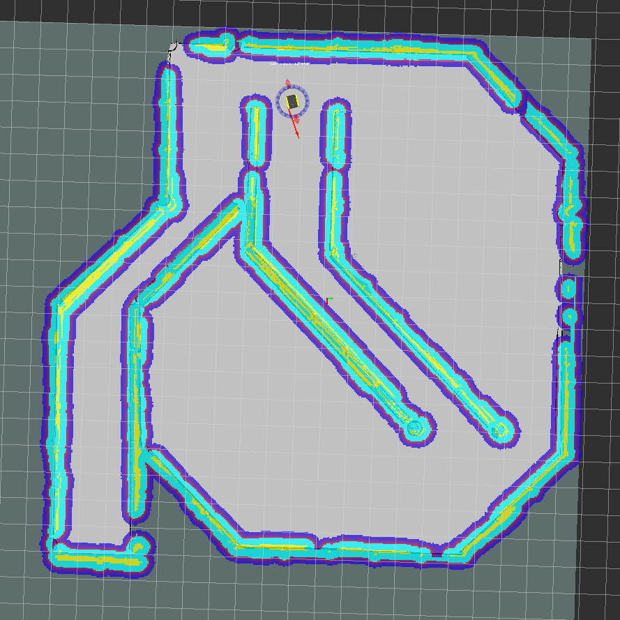
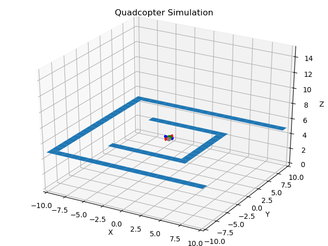
Launch the simulator. The visualizer node already subscribes to the /map topic and displays the map. You should see the map loaded in with obstacles shown in blue, the current waypoint as a grey dot, and the drone as a green dot.

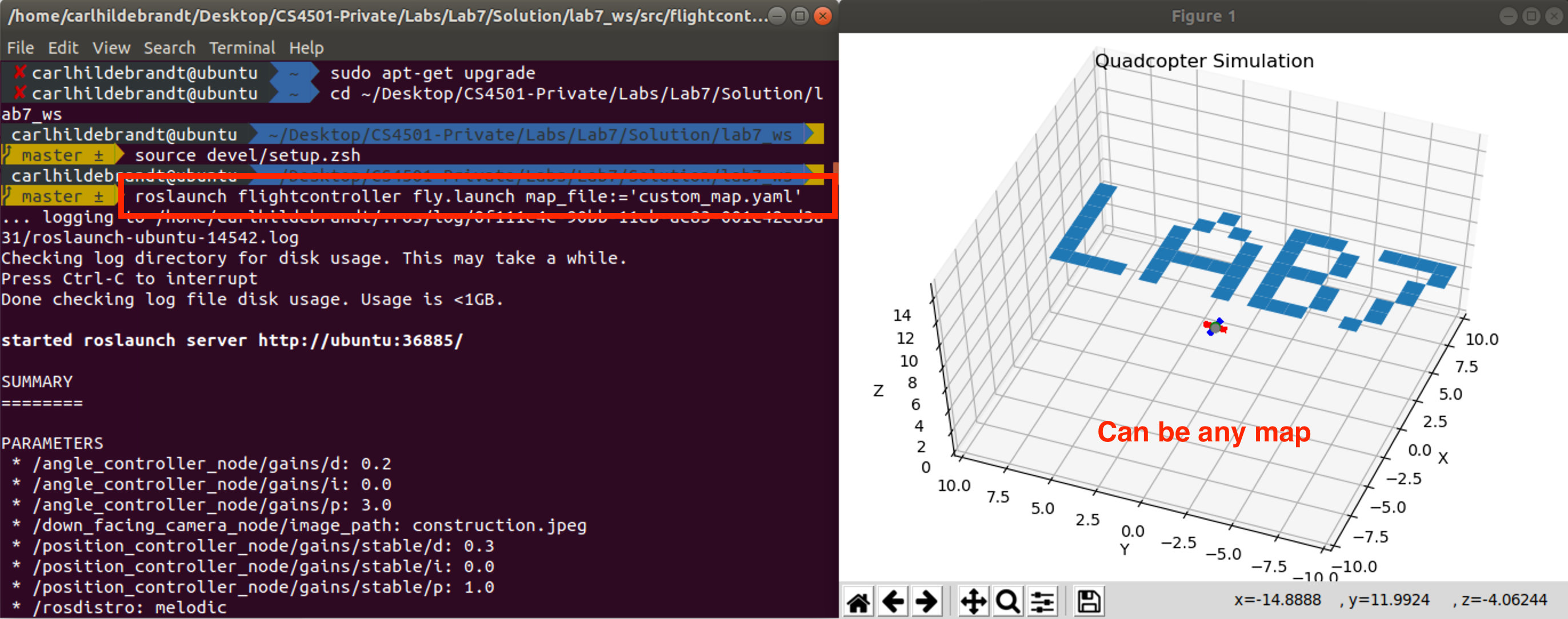
Custom Maps
Now that we can load maps, let’s change our system so that it can load any given map file from the command line. We have provided you with five different map files (four of which are shown later) that can be found here:
$ ls ~/CS4501-Labs/lab7_ws/src/flightcontroller/maps
Now, we want to design our system so that maps can be easily loaded into the simulator.
Adding Arguments to the Launch File
Our launch file has hard-coded the map argument as follows:
args="$(find flightcontroller)/maps/map_medium0.yaml"
This command first finds the flightcontroller packages path and then hard-codes the /maps/map_medium0.yaml to this path. We can make this dynamic by changing the map name to a launch file argument as follows:
args="$(find flightcontroller)/maps/$(arg map_file)"
In this case, we start by finding the path to the package flightcontroller using $(find flightcontroller) and then append the path /maps followed by an argument called map_file using $(arg map_file). The final step is to expose the argument map_file such that we can change that variable from the terminal. To do this add the following line to the top of our launch file
<?xml version="1.0"?>
<launch>
  <arg name="map_file" default="map_medium0.yaml"/>
  ...
This declares that we are creating an argument named map_file and that the default value for this variable is map_medium0.yaml.
Let’s check that we set up everything correctly by launching the system and not declaring the map_file variable instance. It should default to map_medium0.yaml and we should see what we saw in the self-checkpoint. Launch the simulator using:
roslaunch flightcontroller fly.launch
Finally, let’s check that we are able to change the argument using:
roslaunch flightcontroller fly.launch map_file:=map_medium1.yaml
Below we have included what four of the 5 different map files should look like in the simulator.
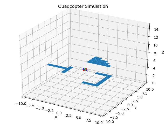
map_medium0.yaml
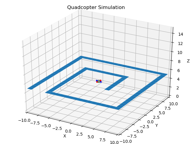
map_medium1.yaml
map_medium2.yaml
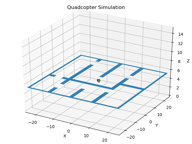
map_large0.yaml
Understanding Map File Formats
Remember when we were reading the map_server wiki page we noticed that they talked about pairs of map files:
.yaml→ Describing the metadata of the map.png→ Describing the occupancy grid data file
The second file is an image format. When we use a common file format we can visualize the map using any standard image viewer. For instance, navigate to the maps directory ~/CS4501-Labs/lab7_ws/src/flightcontroller/maps/. Open each of the map files and you should see:

map_medium0.yaml

map_medium1.yaml

map_medium2.yaml

map_large0.yaml
Now let’s look inside the map_medium0.yaml metadata file:
image: map_medium0.png
resolution: 1
origin: [-10.0, -10.0, 0.0]
occupied_thresh: 0.65
free_thresh: 0.196
negate: 0
The file declares 6 attributes:
- image: filename of the corresponding map
- resolution: resolution of our file where. In our maps, for example, each pixel represents 1 meter.
- origin: pixel at the origin. In our case each map is only 20 pixels wide, thus the origin is the center [-10, -10].
- occupied_thresh: threshold above which declares that a cell is occupied.
- free_thresh: threshold under which we assume the cell is obstacle-free.
- negate: we can use this to invert the map and read white spaces as obstacles and black spaces as obstacle-free.
Now that we have looked at the YAML file, we understand why the map looked so small when we opened them. It was only 20 pixels large, but each pixel represents a large space.
Creating our own Map
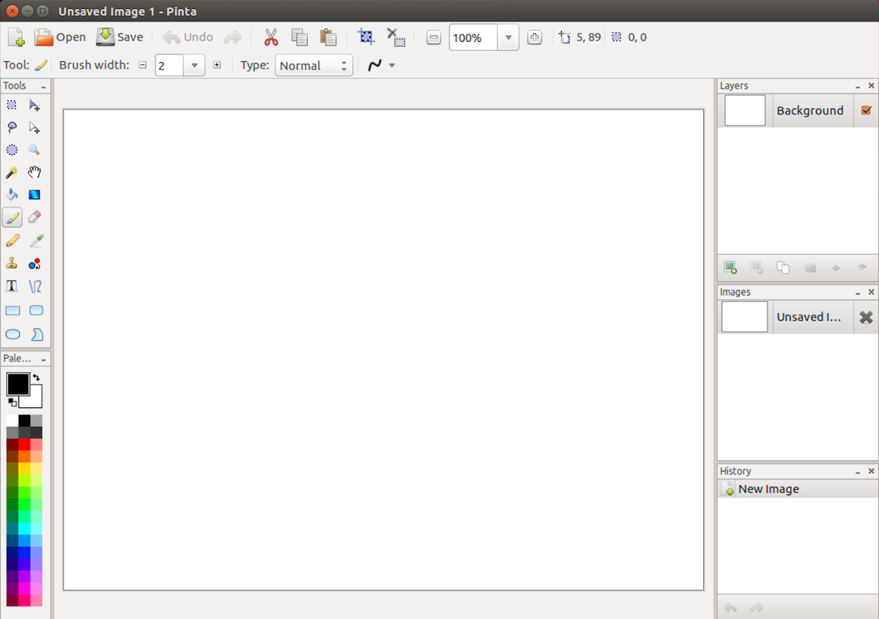
Another benefit of representing maps as images is that we can use standard image processing tools to create our maps by hand. Of course there are other ways of creating maps, such as populating them using the robot’s sensors. However, it might be useful to know how to create maps by hand if you want to test specific scenarios. To do this, we are going to use a free image processing tool in Linux called Pinta. Pinta is similar to Paint that comes with Windows. Note: If you feel more comfortable using another image processing tool, feel free to use that.
Let’s start by installing Pinta. To do that, we run the following commands:
sudo apt-get install software-properties-common
sudo add-apt-repository ppa:pinta-maintainers/pinta-stable
sudo apt-get update
sudo apt-get install pinta
We can then launch Pinta using the command line
$ pinta
You should screen like this:
Start by resizing the window. We are going to make this map of 30 pixels X 30 pixels. You can do that using the drop-down:
- image → resize image → by absolute size
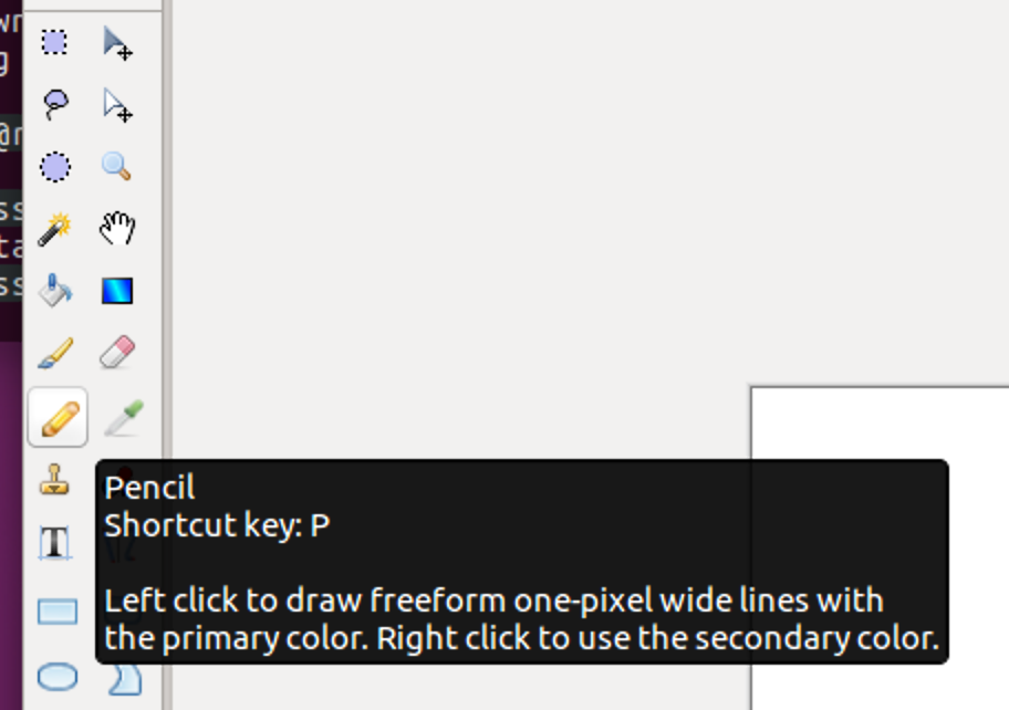
Uncheck the maintain aspect ratio, and then change the width and height to 30 pixels. Zoom in so that you can work on that image. Next, under tools, select the pencil so that we can draw our new map. The pencil can be found as shown below:
Finally, draw a map. In class, you recently learned Bug Algorithm 1, which can be described using the pseudo-code below:
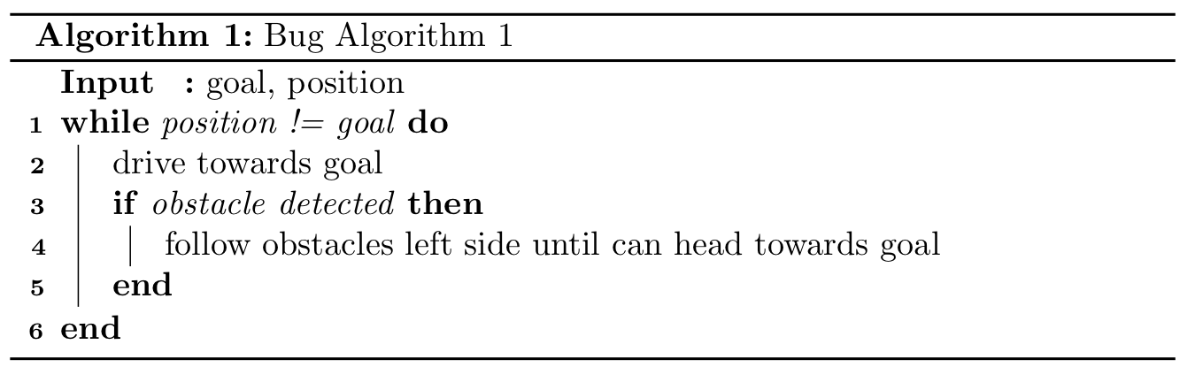
Draw a map that will cause this algorithm to fail. Make sure to leave the central area blank, as this is where your drone will spawn. Once you are done drawing your map, save the map in the correct folder using file → save as. Now that we have our new map file, the final step is to create the corresponding YAML file with the map specifications as follows. Save the YAML file using the same name as your image file with the yaml extension. Using what you have learned, fill in the TODOs section of the yaml file.
image: TODO
resolution: 1
origin: [TODO, TODO, 0.0]
occupied_thresh: 0.65
free_thresh: 0.196
negate: 0
Checkpoint 1
Launch the simulator with the custom map. You should be able to:
- Launch the custom map using the command line.
- Explain why this map could cause bug algorithm 1 to fail.
From Grids to Graphs
Now that we can load maps, we will learn how to navigate them.
In class, we learned that we could create paths through a map by converting the problem into a graph searching problem. There is one problem with our setup right now: our maps are currently represented as a grid. The good news is that a grid can be easily represented as a graph. Look at the grid below. You will notice that we can represent each cell as a node and then add edges to each adjacent cell.

Using this new understanding of grids, we can easily convert our map into a graph. Our map represents free space using 0, and obstacles using 100. Thus, for cells with value 0, we should construct edges to all adjacent nodes that have a value of 0. Moreover, because we are using a drone, we will assume that we can fly diagonally, so we can even connect 0-value cells diagonally. Therefore, our occupancy grid can be converted into a graph as shown below:
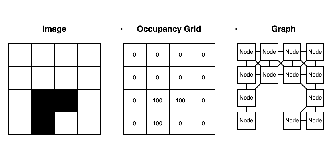
The set of edges in this graph contain all feasible cell-to-cell paths that the drone could take in our environment. With this knowledge, we can now start to implement the graph searching algorithm, enabling our drone to navigate through our maps.
Finding a Path
For the next part of this lab, we will use the map to plan a route from our drone’s position to a set goal.
We will be using the A* pathfinding algorithm to help navigate the drone around the map. A* works by favoring open grid cells (“nodes” in our graph) that are deemed the most promising for reaching the goal, according to some heuristic. This heuristic could be a function that determines the distance to the goal, the time to the goal, or even the forces applied to the vehicle. In our case, we will define the heuristic as the Euclidian distance to the goal. An animated example of the A* algorithm (that favors nodes closer to the goal) is shown below. It first explores nodes leading you in the direction of the goal. Once it hits an obstacle, it slowly expands its search until it finds a path around the obstacle and then continues toward the goal.
The color indicates their distance to the goal (greener is closer and red is farther), and open blue nodes are candidate nodes that have not yet been explored.
To start the implementation of our algorithm, we will create a node path_planner that controls the flow of our implementation. The node will subscribe to the map, current position, and goal. Once the node has this information, it will search the graph for the shortest path and then publish a requested position and a path.
The path_planner node is already provided in the simple_control package. The package also contains the Python class astar_class.py, in which you will implement the A* algorithm.
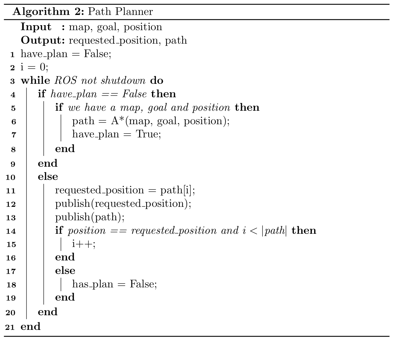
To understand how the path_planner works, let’s follow the pseudocode below. Its takes as input a map, a goal, and the robot position. It initializes variables in lines 1 and 2, and then it iterates until the ROS code is shutdown. In line 4 it checks whether there is a plan generated. If there is no plan and the parameters are valid, it invokes A* to generate a plan in line 6. Once the algorithm has a plan, line 11 gets the next waypoint in the path and publishes both the waypoint and path in lines 12 and 13. Line 14 checks if the drone has reached the requested position and if there are still more points in the path. If these conditions are met, then the next waypoint is retrieved. If the conditions are not met, we reset the has_plan variable.
Your job will be to implement the A* search algorithm class (shown below). You will notice that inside the given path_planner node in the simple_control package, you can see the following lines:
from astar_class import AStarPlanner
...
astar = AStarPlanner(safe_distance=1)
path = astar.plan(self.map, self.drone_position, self.goal_position)
These lines create an astar class object and then use the member function plan to create the path. Your job will be to complete the Python class astar_class.py (found in the src folder of the simple_control package). The skeleton code for this class is shown below (shortened for presentation here):
...

class AStarPlanner:
  # Initilize any variables
  def __init__(self, safe_distance=1):
    ...

  # Find a plan through the map from drone_position to goal_position
  def plan(self, map_data, drone_position, goal_position):
    # Validate the data
    self.validate_data(map_data, drone_position, goal_position)
    # Expand the obstacles by the safety factor
    map_data = self.expand_obstacles(map_data, self.safe_distance)
    ...
    # TODO
    ...

  # Get the children nodes for the current node
  def get_neighbors(self, node_in, map_in):
    ...

  # Validate the incoming data
  def validate_data(self, map_data, drone_position, goal_position):
    ...

  # Expand the obstacles by distance so you do not hit one
  def expand_obstacles(self, map_data, distance):
    ...
Inside the skeleton code, we have implemented three functions for you. The first function is get_neighbors. This function takes in a node’s position and the map, and returns all the neighbors of that node. The second is called validate_data. This function is used for asserting that all data passed to the function is valid. The third function is called expand_obstacles, which expands all obstacles by a set value to give us a wider margin around the obstacles so we do not fly into any obstacle accidentally while traversing the map. For example, even though the drone can fly diagonally, if we were to try to fly directly around a corner we might clip the obstacle, etc. This also helps avoid edge cases where two corners meet.
The plan function returns a list of lists. For instance to traverse from the point [15, 15] to [13, 14] you will return the path [[15, 15], [14, 14], [13, 14]].
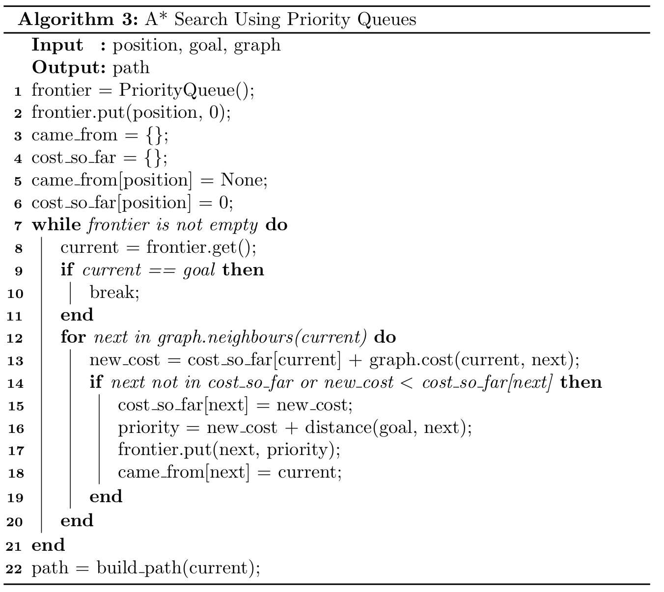
There are many ways to implement the A* search algorithm. Python has a wide range of supporting data structures you may want to use (for instance, PriorityQueues, Lists, Dictionaries). For this reason, the given code has been left bare to allow you to implement the algorithm however you see fit. For example, your implementation could use lists, priority queues, dictionaries, etc. to keep track of the frontier and nodes which had been visited. Use whichever data structures you feel most comfortable with.
Below is the pseudocode for implementing the A* Algorithm using PriorityQueue’s. Note that the “cost” between nodes is simply the Euclidean distance between them.
Testing your Search Algorithm
As in previous labs, we have provided you with some unit tests to test your python A* class available in ~/CS4501-Labs/lab7_ws/src/simple_control/src/test_astar.py. We provide four test cases:
test_straight_x: checks if the goal is placed in a straight line along the x-axis with no obstacles. We expect the path to move directly there in a straight line.test_straight_y: checks if the goal is placed in a straight line along the y-axis with no obstacles. We expect the path to move directly there in a straight line.test_diagonal: checks if the goal is placed along a diagonal line along both the x and y-axis with no obstacles. We expect the path to move directly there along a diagonal line.test_obstacle: checks if the goal is placed in a straight line along the y-axis with an obstacle in between. We expect the path to lead around the obstacle taking the path with the shortest length to the goal.
You can use these unit tests to validate and help you debug your A* search class.
To run the tests, execute the following command.
$ cd ~/CS4501-Labs/lab7_ws/src/simple_control/src
$ python2 test_astar.py
While it is running, open your VNC browser to visualize each test. After clicking out of each window, if all tests pass, you should have the following output:
Note: Make sure to use Python2 as this is the version of python that ROS uses.
>>>....
>>> ----------------------------------------------------------------------
>>> Ran 4 tests in 0.062s
To make sure your implementations is working correctly, you will need to add two additional tests. The first test should test that your algorithm can backtrack. The second test should test if your code works for very long paths (to check for any memory leaks). Remember that the expand_obstacles function in the A* implementation will add extra padding from the obstacles defined in the test.
Once you are sure your code works, you should be able to launch the simulator and send it a goal. You can do that as follows:
Terminal 1:
$ roslaunch flightcontroller fly.launch map_file:=map_medium0.yaml
Wait a few seconds until the drone has started. Then, in Terminal 2:
$ rostopic pub /uav/input/goal geometry_msgs/Vector3 '{x: -2, y: -1, z: 5}'
The second terminal will publish the goal, which will invoke the A* planner. Note: Be certain that your goal is set to an open cell in the map.
You might notice that we are requesting a negative x and y as a goal. In our python unit tests, these would have returned errors, as you cannot request a negative pixel value. The reason we can do this here is because of a transformation from the pixel-based coordinate system used by the map to the spatial coordinate system used by our system. The center of a map, which is 20x20 pixels wide, is [10,10]. However, the drone starts in the center of the simulation, which is [0,0]. Thus when we request the position ‘{x: -2, y: -1}’, this is transformed by the path_planner to the map coordinate system, which would be [8,9]. If this does not make sense, do not worry, this is done for you in this lab, and will be covered in more detail in Lab 8.
Checkpoint 2
To complete this checkpoint you need to:
- Show that your unit tests pass.
- Explain how you implemented the other unit tests, and how do they test the required specifications (backtracking, and length).
- Show that you can compute a path and that the drone will traverse it as shown below:
Specifically launch the small map by running:
$ roslaunch flightcontroller fly.launch map_file:=map_small0.yaml
Then fly to three different goals. Run the following commands:
$ rostopic pub /uav/input/goal geometry_msgs/Vector3 '{x: -4, y: 0, z: 5}'
$ rostopic pub /uav/input/goal geometry_msgs/Vector3 '{x: -2, y: 2, z: 5}'
$ rostopic pub /uav/input/goal geometry_msgs/Vector3 '{x: 4, y: -2, z: 5}'
Editing Obstacle Safe Distance
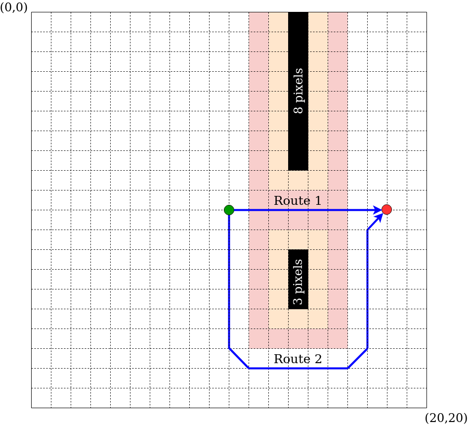
As a final checkpoint, let’s experiment with how the obstacle window size plays a part in the drone’s navigation. Start by creating a [20, 20] pixels wide map with two groups of obstacles. The first is 8 pixels long and goes to the edge of the map. The second is 3 pixels long and creates a gap of 4 pixels between it and the 8 pixel obstacle (as shown below).
Once you have created the map, update the path_planner node to take in a ROS parameter that defines the safe distance (integer value) away from obstacles. Use this parameter to update the following line in the path_planner.
# TODO Update to use a launch parameter instead of static value
astar = AStarPlanner(safe_distance=1)
Instead of using a static safe_distance of 1, set the distance to the new parameter you defined. Once you have added the new parameter and updated the AStarPlanner to use this parameter, add the parameter to the fly.launch so that you can change it at launch. Test your code for different distances. The above image shows two different shades around the obstacles, with the orange representing a safe distance of 1, and the red representing a safe distance of 2. When the distance is large enough, the AStarPlanner will not see the route between the obstacles as safe, and instead, go around the obstacles.
Checkpoint 3
- Showcase your drone flying between the obstacles when the
safe_distanceis set to 1. - Showcase your drone flying around the obstacles when you use a larger
safe_distance.
Congratulations, you are done with lab 7!
Final Check
- Launch the simulator:
- Launch the custom map using the command line.
- Explain why this map could cause bug algorithm 1 to fail.
- Verify that your path planning works
- Show that your unit tests pass.
- Explain how you implemented the other unit tests, and how do they test the required specifications (backtracking, and length).
- Show that you can compute path and that the drone will traverse it.
- Add the
safe_distanceas a launch parameter, and create a map with gap created by two obstacles.- Showcase your drone flying between the obstacles when the
safe_distanceis set to 1 - Showcase your drone flying around the obstacles when you use a larger
safe_distance.
- Showcase your drone flying between the obstacles when the