Hint: You have two options to do this: use rospy.rate which attempts to run your loop at the frequency provided by waiting on the line rospy.sleep. A better approach would be to use python’s built-in time function to measure the time the drone has been waiting at a given position.
Interpreting Rich Image Data
Consider all the information we acquire when driving down a highway. Through our eyes, we sense a stream of images to interpret lane markings, potential obstacles, road signs, other vehicles, their intentions through their brake lights and blinkers, the road condition, and even animals that might try to cross. In robotics, different types of cameras provide an extremely rich source of information. Autonomous vehicles, for example, use one or multiple cameras (and a battery of other sensors) to sense the world. The interpretation of this data is performed by a perception layer that relies on specialized processing techniques and machine learning. We will examine the perception layer through this lab.
Learning Objectives
At the end of this lab, you should understand:
- How to use RQT to view images.
- How to add command-line arguments into a launch file to give input to the robot during startup.
- How to employ basic image processing techniques for object identification.
- How to use ROS’s image bridge to publish and receive images over topics.
- How to train machine learning algorithms to classify detected objects.
Overall Scenario for the Lab
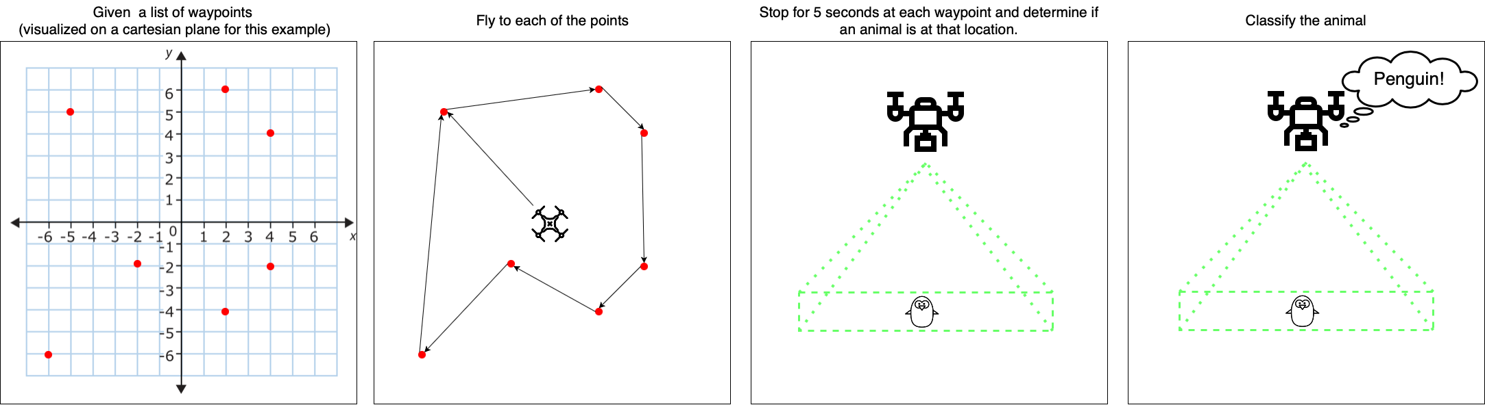
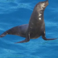
In this lab, we will be developing a drone subsystem that will serve a marine life conservation effort by providing automated and accurate counts of the many marine animals in a target area. Your system already has support for basic navigation to a waypoint, an altitude controller, and a downfacing camera.
For each mission, the conservationist will set locations they want the drone to check. As an example, the marine conservationists give you 7 locations where a single animal might be. Your drone is to fly to those checkpoints (For this lab, if an animal is spotted during traversing between waypoints, it can be ignored). Once at a location, your drone should wait there for 5 seconds. During this time, it needs to use a perception node to determine if there is an animal at the location. If an animal is detected, your drone should decide which type of animal it is before moving to the next waypoint. The conservationists inform you that you are most likely to see dolphins, penguins, and seals.
Prerequisites
We will be using additional Python libraries in this lab that are not installed on the original docker image that you are using. Before you continue, please update the docker container using the commands below. This may take a few minutes to build; during that time you can work on writing the code that is required for Checkpoint 1.
NOTE: the git pull may fail because you have made changes to your docker-compose.yml to adjust the resolution as discussed in Lab 1. If this is the case, you should write down what resolution you had, then run git checkout docker-compose.yml to reset the file. Then, you can use git pull to get the updates, and then manually edit docker-compose.yml to adjust the resolution back.
cd ~/cs4501-robotics-docker # Or wherever you have the docker repo set up
docker-compose stop # Stop the docker so we can update it
git checkout main # Ensure you are on the main branch
# Download the new docker configuration and rebuild the docker image. This may take several minutes
git pull && \
docker-compose up --build -d || \
echo "Git pull unsuccessful, docker-compose not run. Address issues and try again."
Part 1: Getting to Identify the Animals
The first step is to get the drone to fly to the specified possible animal locations. Once we have done that, we need to develop a perception node that can identify whether an animal is at each location.
Controlling the Drone Movement
We will start by creating a node that tells the drone to fly to a set of predefined positions (we will later edit this node so that a user can update those waypoints from the command line). The code skeleton with the functionality for flying between waypoints is in the node visit_waypoints.py in the simple_control package. To make a drone fly to a waypoint, we need to publish a waypoint as a Vector3 on the topic /uav/input/position_request. We will also need to subscribe to the topic uav/sensors/gps to check whether the drone has arrived. The drone should wait 5 seconds before moving onto the next waypoint. To determine the time between waypoints, we should calculate the elapsed time. Another option is to use ROS rate which fixes the frequency of the loop to 1Hz. However, in general, this is not a safe way to implement timing, as many of these functions work on a “best-effort” basis. That means if something were to happen and the computer could not maintain the 1Hz, it would continue as if nothing happened, making your timing information incorrect.
# A class used to visit different waypoints on a map
class VisitWaypoints():
  # On node initialization
  def __init__(self):
    # Init the waypoints [x,y] pairs, we will later obtain them from the command line
    waypoints_str = "[[2,6],[2,-4],[-2,-2],[4,-2],[-5,5],[4,4],[-6,-6]]"
    # Convert from string to numpy array
    try:
      self.waypoints=waypoints_str.replace('[','')
      self.waypoints=self.waypoints.replace(']','')
      self.waypoints=np.fromstring(self.waypoints,dtype=int,sep=',')
      self.waypoints=np.reshape(self.waypoints, (-1, 2))
    except:
      print("Error: Could not convert waypoints to Numpy array")
      print(waypoints_str)
      exit()

    # Create the position message we are going to be sending
    self.pos = Vector3()
    self.pos.z = 2.0

    # TODO Checkpoint 1:
    # Subscribe to `uav/sensors/gps`

    # Create the publisher and subscriber
    self.position_pub = rospy.Publisher('/uav/input/position_request', Vector3, queue_size=1)

    # Call the mainloop of our class
    self.mainloop()

  def mainloop(self):
    # Set the rate of this loop
    rate = rospy.Rate(1)

    # Wait 10 seconds before starting
    time.sleep(10)

    # TODO Checkpoint 1
    # Update mainloop() to fly between the different positions

    # While ROS is still running
    while not rospy.is_shutdown():

      # TODO Checkpoint 1
      # Check that we are at the waypoint for 5 seconds

      # Publish the position
      self.position_pub.publish(self.pos)

      # Sleep for the remainder of the loop
      rate.sleep()


if __name__ == '__main__':
  rospy.init_node('visit_waypoints')
  try:
    ktp = VisitWaypoints()
  except rospy.ROSInterruptException:
    pass
Adding Command Line Arguments
A good practice with ROS is to expose your ROS code inputs as parameters in a launch file. That way, they can easily be changed without the need to recompile your code. Additionally other developers who use your code can easily identify which values are meant as input. An example of this is the waypoints we want to send to the drone. Each time we fly, we might want a different set of waypoints, and by moving them to the launch file we make it clear that this is input to our program. Another benefit of moving variables to parameters in the launch file, is that it allows us to expose them to the command line. That way we can enter the input from the command line and avoid editing the launch file altogether.
To start this section, first let’s change the hardcoded waypoints to parameters which we can set in our launch file. To do that update the waypoint_str definition to:
waypoints_str = rospy.get_param("/visit_waypoints_node/waypoints", "[[2,6],[2,-4],[-2,-2],[4,-2],[-5,5],[4,4],[-6,-6]]")
By doing this we have now allowed our waypoints to be set using the parameter /visit_waypoints_node/waypoints. Next update the fly.launch launch file as follows:
<?xml version="1.0"?>
<launch>

  <arg name="search_image" default="test1.jpg" />
  <arg name="waypoints" default="[[2,6],[2,-4],[-2,-2],[4,-2],[-5,5],[4,4],[-6,-6]]" />

  <include file="$(find flightgoggles)/launch/core.launch">
  </include>

  ...

  <node name="visit_waypoints_node" pkg="simple_control" type="visit_waypoints.py" output="screen">
    <param name="waypoints" type="string" value="$(arg waypoints)" />
  </node>
  <node name="perception_node" pkg="perception" type="perception.py" output="screen"/>

</launch>
We have now declared a new argument for our launch file called waypoints. The default value for this argument is the list of waypoints that were given to us by the conservationists. We have also updated the visit_waypoints_node to include the parameter /visit_waypoints_node/waypoints of the type string. We then set the value of this parameter to the argument of the launch file waypoints. By doing this we can now set out waypoints using the command line as follows:
roslaunch flightcontroller fly.launch waypoints:='[[-4,-1],[2,6],[2,-4],[4,-2],[-5,5],[4,4],[-6,-6]]'
Using RQT to View Image Data
Now that the drone flies between the different positions on the map, let’s see if we can manually spot an animal. RQT provides you with a view of the camera data sent on a topic.
Start by launching the drone. In another terminal launch RQT, click Plugins->Visualization->Image View, and select our camera topic uav/sensors/camera from the dropdown. You should see something like is shown below:
The drone is autonomously navigating to different parts of the map while we get to view the camera data using RQT (note that to speed up the demonstration, our drone only stayed at each waypoint for 1 second)
Checkpoint 1
Show that your drone continuously flies between points in the following sets of waypoints:
- Waypoint set 1:
'[[2,6],[7,0],[4,-2],[-6,-6]]' - Waypoint set 2:
'[[-4,-1],[2,-4],[-7,0],[4,4]]'
- Show that your drone navigates to each of the waypoint sets while displaying the RQT image view. See if you can manually spot an animal.
- Show your drone waiting at each waypoint for 5 seconds.
- Explain how you implemented the
visit_waypointsnode.
Using Image Processing for Object Identification
Let’s now use the downfacing camera to identify when an animal is in the picture frame automatically. To implement this function you will use OpenCV. OpenCV (Open Source Computer Vision Library) is an open-source library of over 2500 algorithms including a comprehensive set of both classic and state-of-the-art computer vision and machine learning algorithms. We will start by developing a python class, MarineLifeDetection (independent of ROS for now). This class has 3 main functions:
create_marine_life_mask: Creates a mask by color thresholding the image. The input is an image and the output is a mask.segment_image: Segments the image using the mask so that it only contains the animal. The input is a mask and the output is an image.marine_life_detected: Determines if an animal was detected by looking at the ratio of white/black pixels in the mask. The input is a mask and the output is a boolean value.
The 3 functions you will need to implement are in the marine_life_detection.py file, inside the perception package. To aid in developing this class, we have provided a debug script,debug_detection.py, which calls these functions using sample images. Thus, for debugging your code, you can run the command:
cd ~/CS4501-Labs/lab5_ws/src/perception/src
python debug_detection.py
This debug script will automatically load an image and pass it to the respective functions (similar to what you will need to do when implementing it in ROS). The provided script loops through 8 different images, each in .jpeg format.
It generates an HSV (Hue, Saturation, Value) plot which can be used as described below. Next the script calls the functions you will need to implement create_marine_life_mask, segment_image, and finally marine_life_detected. It then displays the raw image, the segmented image, and whether an animal was detected. The debug code is shown below.
def debug_hsv(image, fig):
    # Omitted for brevity

# Create the marine life detection class
d = MarineLifeDetection()

# For the 8 test images
for i in np.arange(1, 8):

  # Load the test image
  image = cv2.imread('../test_data/test' + str(i) + '.jpeg')

  # Convert to smaller size for easier viewing
  img = cv2.resize(image, (200, 200))

  # Create a figure showing the HSV values
  fig = plt.figure(1)
  h,s,v,pixel_colors = debug_hsv(img, fig)
  plt.pause(0.05)

  # Use the marine life detection class functions
  # NOTE: These are the functions you will need to implement
  mask = d.create_marine_life_mask(img)
  seg_img = d.segment_image(img, mask)
  detected = d.marine_life_detected(mask)
  print("Animal Detected: " + str(detected))

  # Display returned images
  if img is not None:
    cv2.imshow('Raw Image',img)
  if seg_img is not None:
    cv2.imshow('Marine Life', seg_img)

  # Wait 5 seconds before continuing the loop
  key = cv2.waitKey(5000)
  if key == 27:
      cv2.destroyAllWindows()
      break

cv2.destroyAllWindows()
Color Threshold
In the lecture, we introduced the idea of using HSV for color segmentation. Let’s apply it here. HSV represents the colors in a cylindrical format, making it easy to segment the image based on color. The function debug_hsv() inside the debug_detection.py file already plots the HSV values of an image so that you can identify the colors that are not associated with marine animals.
Below we walk you through an example of how to do this. Let’s assume we wanted to isolate the orange frog. The goal is to create an image where only the frog is shown by removing all colors other than orange.
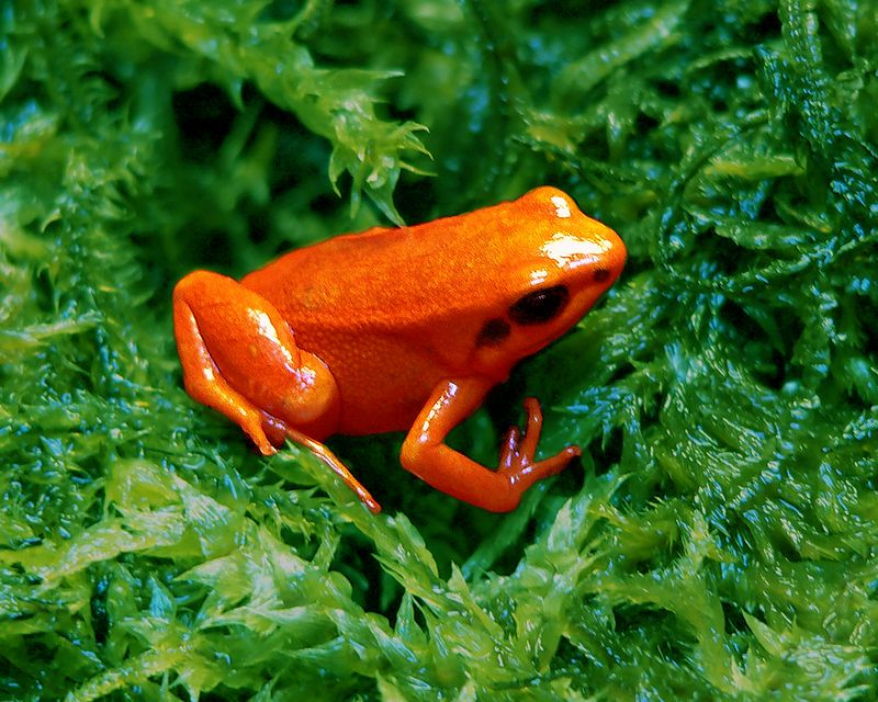
Source: The original image showing all colors.

The desired output where we have removed all colors other than orange.
If we were to pass this image to our debug_hsv() function inside the debug_detection.py file, we would get the plot shown below. Using this plot, we can identify which range of HSV values contains the orange pixels. For example, using the plots below, we identify that the orange pixel values lie in the HSV range H=[0, 25], S=[100, 255], V=[100, 255].
Note: To change the viewing angle of the plot use the function axis.view_init(0, 0) in the debug_hsv function.
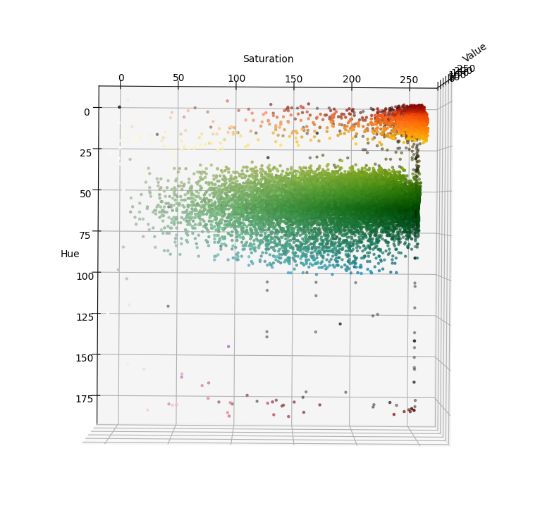
Saturation vs Hue
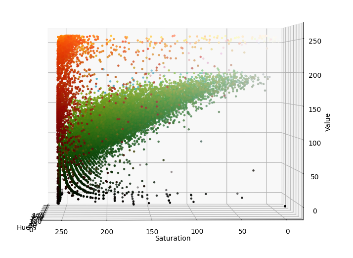
Saturation vs Value
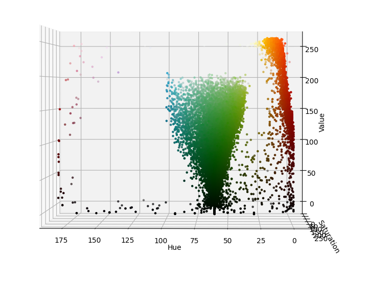
Hue vs Value
Following a similar process to obtain the marine animals’ values, you can now implement the function create_marine_life_mask in marine_life_detection.py file. The pseudocode is as follows:
def create_marine_life_mask(self, image):
    # Convert the image to the HSV format using opencv
    # Define your HSV upper values
    # Define your HSV lower values
    # Generate a mask using opencv inrange function.
    # Return the mask
The resulting mask is a 2D array with the same width and height as our image. Each cell in the mask has a value between 0 and 255. The value 0 is displayed as black, and the value 255 is displayed as white. Each black pixel represents a pixel in our original image that is outside the defined color range. Every white pixel represents a pixel within the defined color range in our original image. The mask for the previous frog is shown below:
The orignal image showing all colors.
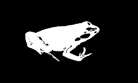
A mask which highlights all orange colors.
One way to check that our color isolation function is working is to plot only the mask’s pixels that are not removed. To do this we will develop the function segment_image() in marine_life_detection.py file. The function should return black pixels where the mask is 0, and return the original pixel when the mask is 255. A quick and efficient way of doing this is using a bitwise_and operation. The function is described below:
def segment_image(self, image, mask):
  # Return the bitwise_and of the image and the mask. Note opencv has a bitwise_and operation
  # Return the resultant image
Object Identification
We now have a mask that tells us which pixels in the original image are within the target color range. The mask can also tell us how many pixels in the image may be associated with the animals in question. Given our previous experience capturing animals at the set altitude with this camera, we can then use a simple threshold to determine if the ratio of animal pixels compared to all pixels is high enough that we are confident we may be looking at an animal (this is not a great mechanism, but it should suffice as a coarse approximation for now). Implement a function that computes the ratio of animal pixels to all pixels in the mask image (i.e. compute the ratio of 0 vs 255 pixel values). Then find a threshold for this ratio which reliably returns whether an animal detected, this might take some trial and error. You can implement this in the marine_life_detected in marine_life_detection.py file. The function is described below:
def marine_life_detected(self, mask):
  # Compute the size of the mask
  # Compute the number of marine animal pixels in the mask
  # Use the ratio of these values to determine whether an animal was detected or not
  # Return whether an animal is detected or not
Once all three functions are implemented, you should see something similar to the output when running debug_detection.py. Note in the actual code, some of the debug images do not contain a animal. In these cases it should return false.
Testing your Code
Although we have provided you with a debugging script, it is always good software engineering practice to test your code. We have provided you with unit tests that you will need to run to check that your functions work. Before you run these tests, make sure you have implemented each of the required functions as described above. Once you have debugged your code and think it is working, we have provided a test_detection.py script that uses unit tests to test whether your functions are implemented correctly. We will use this script to assert that your functions detect the animal if an image contains an animal. To run the unit tests, you can use:
Note: The -m option tells unittest to load a file. Therefore you do not need to include .py. More information about this can be found here.
python -m unittest test_detection
Below is the output of the unit tests if all tests passed:
>>> ----------------------------------------------------------------------
>>> Ran 8 tests in 0.064s
Checkpoint 2
Implement functions in the marine_life_detection.py class located in the perception package. Remember, an easy way to debug your code is to use python debug_detection.py when in the perception/src directory. Once you are sure your code is working, test it using test_detection.py when in the perception/src directory.
- Showcase that your functions work correctly by running the unit tests.
- What other technique could you use to achieve similar results?
- Explain how you determined if an animal was present using the mask. What threshold did you use, how to determine the best value to use?
- When would your technique not work?
Integration into ROS code
As we saw earlier, our drone has a downfacing camera taking images of the surface below it. These images are transported on the topic /uav/sensors/camera. ROS transports messages using its own sensor message format, sensor_msgs/Image. However, we have started to learn the power and versatility that OpenCV provides in image processing. Due to this, many developers use OpenCV’s image format instead of the ROS one. CvBridge is a ROS library that provides an interface between ROS and OpenCV. CvBridge provides transformations between the two formats and is extremely useful when working with images in ROS.
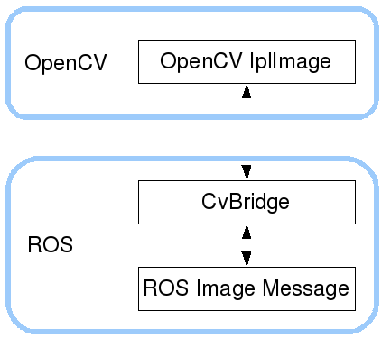
When we receive a message of type sensor_msgs/Image, if we want to work with it using OpenCV, we first need to pass it to the CvBridge class for encoding. To convert a ROS message into OpenCV’s image format, you can use the following code:
from cv_bridge import CvBridge
bridge = CvBridge()
cv_image = bridge.imgmsg_to_cv2(image_message, desired_encoding='passthrough')
Similarly, once we are done processing an image and want to publish it as a ROS sensor_msgs/Image, we need to pass it to the CvBridge class for decoding. You can do that using the following code:
from cv_bridge import CvBridge
bridge = CvBridge()
image_message = bridge.cv2_to_imgmsg(cv_image, encoding="passthrough")
More information on CVBridge can be found here.
Now that we know how to convert ROS messages to the OpenCV image format, we can connect our code in marine_life_detection.py to start processing the down-facing camera images. To do this, we have given you a node perception in the perception package. Inside this node, you will see the subscriber:
self.image_sub = rospy.Subscriber("/uav/sensors/camera", Image, self.downfacing_camera_callback)
This subscriber listens to the uav/sensors/camera topic and passes the image to the downfacing_camera_callback function. In this function, you need to convert the image from a ROS sensor_msgs/Image image, to an OpenCV image. Then, pass it to marine_life_detection.py and use the functions we implemented to detect if there is an animal or not.
Use the functions we created in marine_life_detection.py to allow the perception node to detect an animal within the image captured by your downfacing camera. Save this information in the boolean variable self.detected. Publish whether an animal has been detected or not on the topic /marine_life_detected, which is of type Bool.
Checkpoint 3
Showcase the integration of the perception layer into ROS. To do that:
- Showcase your drone traversing the waypoints on a given scenario and autonomously detecting an animal.
- Showcase that your drone publishes that an animal is detected by echoing
/marine_life_detected.
Part 2: Classifying the Animals
Our project’s second part is to develop a subsystem that can automatically classify the animal. To do that, we will train a deep learning model that uses a neural network to classify the animals. Neural networks typically require large amounts of training data to be accurate. One of the ways to gather more data and increase the robustness of your neural network is to take some of your training data and augment it to create new data. These augmentations need to be something that preserves the same meaning of the image while giving the neural network new information to train on. For example, if we have an image of a dolphin, then we could generate an image of an upside-down dolphin as an augmentation. We will cover several types of augmentations below.
This section starts with augmentation strategies to create large amounts of training data, followed by training an existing neural network and finally using it to classify animals.
Create richer training data
A deep learning model’s prediction accuracy largely depends on the amount and diversity of data available during training. Data augmentation can aid in achieving these requirements by generating carefully modified copies of already labeled images. For example, augmentation can rotate an animal’s image, rendering a new image that still holds the same label as the original image.
We have added a machine_learning folder inside the perception node containing create_data.py, which loads 60 labeled images containing marine animals similar to what your drone will see when flying. For our machine learning algorithm to succeed, we will need many more images. The create_data.py script uses a DataAugmentation class located in data_augmentation.py which contains function skeletons to augment the images in different ways:
zoom(optional): Outputs a list of images with different magnification.translate_image(optional): Outputs a list of images with different translations.rotate_image(optional): Outputs a list of images rotated to varying degree.blur_image(required): Outputs a list of images, each blurred differently.change_brightness(required): Outputs a list of images, each with varying brightness.add_noise(required): Outputs a list of images with added random noise.combine_data_augmentation_functions(required): Outputs a list of images with different combinations of the above functions.
Your goal is to implement all of the required functions and one of the optional functions (Note we describe each function in the relevant sections below). Remember, the more data you generate for your network, the better your classification performance will be. We give pseudocode for each of these skeleton functions and point you to the OpenCV documentation where needed. Note there are always multiple ways to implement such functions so take the pseudocode just as guidance. Just remember to check your output to make sure it is what you would expect.
Before we run create_data.py we will need to be sure our data augmentation is working. To help you check whether the data augmentation functions are working, we have provided you with a debug_data_augmentation script. This script will pass a single image into each function and save the resultant images to a folder machine_learning/debug_data. You can then view these images to see if the functions are working as expected.
To run this script you can do the following:
cd ~/CS4501-Labs/lab5_ws/src/perception/machine_learning
python debug_data_augmentation.py
Note: The script does not delete previous data. You should consider removing the prior debug images with rm -r debug_data between runs.
Zooming (Optional)
A drone is continually performing pitch, roll, and thrust adjustments as it attempts to move or even hover at a location. These adjustments cause variations in altitude and in camera angles that may make the animals appear different in the field from what was learned from the training set. To simulate these effects, we have implemented a zoom function. This is one of the more complicated functions, as it requires padding as you zoom out. To keep our function simple, we pad the edges of the image with black pixels. Even better padding would be to pad the image with a pixel color similar to the watercolor. However, for this lab, it is okay to use black pixels as padding for simplicity.
# Create a list to hold the output
# Define the zoom percentages
# For each zoom percentage
    # Get the image shape
    # Compute the new shape based on the zoom
    # Make the image the new shape
    # Pad or crop the image depending on original size
    # Save new image to list
# Return list
The output from this function looks as follows.

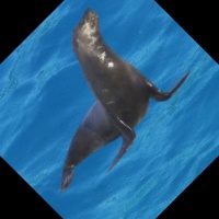
The original image
A zoomed in image
A zoomed out image
Translate an Image (Optional)
Our drone will not necessarily find the animals centered in the camera frame. To account for this variation in our training data, we will create an image translation function. This function will move the center of the image and pad the edges with black pixels. Like the zoom function, better padding would be pixels with a color similar to the water’s color. However, for this lab, it is okay to use black pixels as padding for simplicity. Translating the image will allow the machine learning technique to learn that the animal does not necessarily need to be in the center of the image. Here is the pseudocode you can use to implement this function:
# Create a list to hold the output
# Define the translations
# For each translation in X
    # For each translation in Y
        # Get the current image shape
        # Compute the new shape of the image
        # Warp the image to the new shape
        # Append black pixels to the edge
        # Save the new image
# Return the output
The resultant images from this function will look as follows:
The original image
The image translated to the left and upwards
The image translated to the right and downwards
Image Rotation (Optional)
As animals swim in the water or the drone adjusts its yaw, the animals will appear to rotate in the drone’s camera. To mimic this, we are going to rotate the image. Like the translation and zoom function, we will pad the edges with black pixels as needed (As stated above, we could improve this by using pixels similar to the water’s color pixels). To create this function, you can use the following pseudocode:
# Create a list to hold the output
# Define the rotation we want to consider
# For each rotation
    # Get the image shape
    # Compute the rotation matrix centered around the middle of the image HINT: cv2.getRotationMatrix2D()
    # Warp the image using the rotation matrix
    # Append the image to the output list
# Return the output
You will find the images from this function will look as follows:

The original image
The image rotated 45 degrees
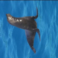
The image rotated 90 degrees
Blurring Image (Required)
As the drone reaches higher speeds moving between points, the images might blur. We thus will augment our data to replicate this real-world phenomenon. Blurring is simple to do in OpenCV with a built-in function blur. This function can be implemented using the following pseudocode:
# Create a list to hold the output
# Define the blur amounts
# For each blur amount
    # Blur the image HINT: cv2.blur
    # Append the image to the output list
# Return the output
Once you are done implementing this function, the output will look as follows:

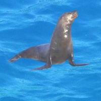
The original image

The image slightly blurred

The image significantly blurred
Changing Image Brightness (Required)
Another natural phenomenon we can consider is light reflecting off the surface of the water. This will change the camera’s exposure to light and distort the image. We can replicate this effect by changing the brightness of the image. We can implement this functionality by converting the image to the HSV format and editing the V component, which directly controls the brightness of the pixel. We then convert it back to the BRG format OpenCV uses when handling images. The pseudo-code can be described as shown below:
# Create a list to hold the output
# Define the brightness levels
# For each brightness level
    # Convert the image into HSV
    # Add the brightness level to the V component
    # Revert to BRG format
    # Append the image to the output list
# Return the output
The output of these images will look as follows:
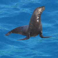
The original image
The image made brighter
The image made darker
Adding Noise (Required)
Another way to create more data and make machine learning techniques more robust is to add noise to the images. This allows the machine learning algorithms to become less reliant on specific pixels in an image to identify what class the image belongs to and look at other aspects of the whole picture. Adding noise is also a good way to train the model on realistic data as sensors in the real world always have some noise. We will add noise by creating a mask of random noise with a specific mean and standard deviation. We can then add that noise to the image to create a new noisy image. This is an easy and effective way of increasing the amount of data you present to your algorithm. The pseudo-code for this function is described below:
# Create a list to hold the output
# Define the mean and sigma values
# For each mean value
    # For each sigma value
        # Create random noise with the same shape as the image HINT: np.random.norma
        # Add the noise to the image
        # Save the new image to the output list
# Return the output
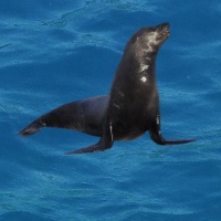
Below we show an example of the original image and the noise. When you add them together, you get the image on the right.

The original image
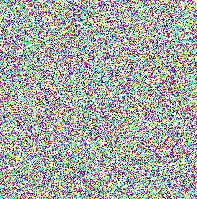
The randomly generated noise
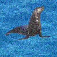
The image and noise added together
Combining your techniques (Required)
Finally, we can implement a technique which combines the implemented functions to create, for instance, noisy rotated blurry images. By combining the underlying transformations, we are able to generate significantly more data to train our system. Create at least 4 unique combinations of functions which combine 2 or more of the above functions.
Creating the data
Once you are sure that you have correctly implemented all of the required functions and 1 of the optional functions, you can generate your new testing data using:
cd ~/CS4501-Labs/lab5_ws/src/perception/machine_learning
python create_data.py
This will create two new folders, namely training_data and testing_data. The folders contain the training and testing data which we will use to train our model to classify the animals.
Train a model
We will now use the augmented data set we just generated to train our machine learning algorithm. In this lab, we will treat the DNN as a black box to be trained, providing you with just an overview of the selected architecture and the code to train it.
Our model is implemented using scikit-learn, a python Machine Learning library. scikit-learn provides a selection of efficient tools for machine learning and statistical modeling including classification, regression, clustering and dimensionality reduction via a consistent interface in Python. For this lab, we are using a relatively simple network to identify the animals. scikit-learn is a great library to use when getting started with machine learning, before moving onto more advanced frameworks like TensorFlow or PyTorch. Before we run the script train_model.py let’s look at the command line arguments which we can use when calling it (these can be found as some of the first lines in the file).
# Check for user arguments
parser.add_argument('--epochs',         type=int, default=25)
parser.add_argument('--batch_size',     type=int, default=64)
parser.add_argument('--hidden_layers',  type=str, default="128,128")
Here we can see that we can set the number of epochs. In machine learning each time a dataset passes through an algorithm, it is said to have completed an epoch. We can define the batch_size. The batch size defines the number of training samples to work through before updating the internal model parameters (which among others means updating the weights). Finally we can describe the number and size of the hidden_layers, the internal dense layers of the neural network.
We have provided a set of default values for these. To get better performance you can experiment with a different number of epochs, a different batch size and even a different network architecture. Note: for the purposes of this lab the defaults should work just fine, except for epochs. If you have less data, each epoch will be computed significantly faster, however you will need more epochs for the weights to have seen enough data to fully update. If you have a ton of data you will need fewer epochs for the weights to be computed, but each epoch will take significantly longer. We found that for 5K training images, you need roughly 200 epochs, while if you have 40K images you only need around 25. Set your number of epochs accordingly. To run the script you can use:
cd ~/CS4501-Labs/lab5_ws/src/perception/machine_learning
python train_model.py --epochs 25 --batch_size 64 --hidden_layers "128,128"
The first thing you will notice when you start training is a summary of the parameters used to train our model:
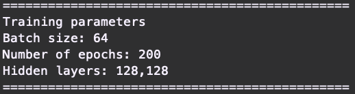
We can see that our model has two hidden layers of size 128 neurons each. Each layer is called a dense layer, where each neuron in the first layer connects with an edge to a neuron in the next layer. This might seem like many edges and parameters which need to be adjusted so that the network can minimize the loss and increase the accuracy. However in reality this is really tiny in comparison to some of the larger networks used in production. For example ResNet152 released in 2015 by Microsoft Research consists of 152 layers, with over 60 million parameters (source).
Break time? The above process to train the DNN might take some time, so go and grab yourself a cup of tea while your computer figures out the best weights to estimate the function to classify the training images with their labels.
Once the training is complete, it will produce a file named model.pkl inside the machine learning folder.
Let’s now look at some of the trained DNN functions. The most important function is our self-defined run_single_image. This function takes in a single image and uses the model to make a prediction on the class of this image. Let’s look at how it works:
# load an image and predict the class
def run_single_image():
    classes = get_classes("./training_data/*/")

    # load model
    print("Loading the model...")
    with open('model.pkl', 'rb') as f:
        model = pickle.load(f)

    # For all images in single_prediction
    sample_images = glob.glob("./testing_data/*.jp*")

    print("\nExecuting on a single image: ")
    for img_name in sample_images:
        # Load the image
        img = cv2.imread(img_name)
        img = cv2.resize(img, (48, 48))
        img = cv2.cvtColor(img, cv2.COLOR_BGR2GRAY)
        x = img.reshape((1, -1))
        x = x.astype('float32')
        x = x / 255.0
        # predict the class
        prediction = model.predict(x)
        result = np.argmax(prediction, axis=-1)
        print('Single image class (' + img_name + '): ' + str(classes[result[0]]))
This function loads the classes 'dolphin', 'seal', 'penguin'. Next, it loads the learned model using pickle.load. Python Pickle is a library used for serializing and de-serializing a Python object structure. In other words you can use it to save python objects and then load them again later on. Finally, we want to test our network on a single image. To replicate the process of classifying images inside the main loop of our node, we create a loop that runs over all test images sample_images. In that loop we convert the image into the format expected by our model. Then we will call predict on the single image and classify it according to the neural network’s prediction.
Integrate into ROS code
The final part of this lab is to integrate your learned model classifier into your codebase. To do that, you need to load the model in the perception node in the perception package. If you detect an animal inside the node, you can pass that image to the model, get the prediction, and publish it to /marine_life_classification topic.
Use the run_single_image function as guidance when implementing this function in ROS. Remember each image in the run_single_image function represents an image received in our callback function. Thus to implement our function in ROS we will first need to load the image. In ROS this is done using CVBridge. Then we use the model.predict function to make a prediction. Our neural network returns the data as an array. The index in the array with the largest value is our predicted class.
More specifically, start by creating a list of classes 'dolphin', 'seal', 'penguin'. Next save the image in the image_callback function so that it can be used inside the mainloop. Then inside the mainloop if an animal is detected, preprocess the image using preprocess_image. We need to preprocess the image so that we can pass it to the model, in the form the model expects. Next pass the new image to the model using the predict function and use argmax over the result to get the class. Publish the class on the /marine_life_classification topic.
Checkpoint 4
Proceed to train your DNN and add it into the perception node.
- Take a screenshot of the training and testing results produced at the end of the training script. We require a testing accuracy of at least 60%.
- Showcase your drone flying to an animal and classifying it.
- Are there cases where your drone incorrectly classifies the animal? Why do you think this is?
Congratulations, you are done with Lab 5!
Final Check:
- Show that your drone continuously flies between points in the following sets of waypoints
'[[2,6],[7,0],[4,-2],[-6,-6]]'and' [[-4,-1],[2,-4],[-7,0],[4,4]]':- Show that your drone navigates to each of the waypoint sets while displaying the RQT image view. See if you can manually spot an animal.
- Show your drone waiting at each waypoint for 5 seconds.
- Explain how you implemented the
visit_waypointsnode.
- Implement the
marine_life_detection.pyclass located in theperception.- Showcase that your functions work correctly by running the unit tests.
- What other technique could you use to achieve similar results?
- Explain how you determined if an animal was present using the mask. What threshold did you use, how to determine the best value to use?
- When would your technique not work?
- Showcase the integration of the perception layer into ROS.
- Showcase your drone traversing the waypoints on a given scenario and autonomously detecting an animal.
- Showcase that your drone publishes that an animal is detected by echoing
/marine_life_detected.
- Proceed to train your DNN and add it into the perception node.
- Take a screenshot of the training and testing results produced at the end of the training script. We require a testing accuracy of at least 60%.
- Showcase your drone flying to an animal and classifying it.
- Are there cases where your drone incorrectly classifies the animal? Why do you think this is?