Image from an Intellias blog post on how self-driving cars use sensors, sensor fusion, and Kalman Filters. This blog post highlights how what you will learn in this lab is used in industry today.
Complex Sensors
Robots have the difficult task of operating in environments that are not completely known and that can change. Sensors provide a window into that world, transforming energy into physical quantities that characterize that world. Depending on the type of robot and its goals, the kind and number of sensors may vary. For example, some simple household robots (e.g. Roomba) are only equipped with a touch sensor to let them know when they bump into walls, while self-driving cars can be equipped with ultrasonics, lasers, multiple cameras, and GPS. The performance of these sensors is affected by many sources of noise that need to be managed, in order to better interpret the world. For example, a camera’s output may noisy due to changes in illumination, high temperatures, conversion from analog to digital signals, and more. In this lab we will explore how sensors are incorporated into a system and how to manage the sources of noise associated with sensors.

Learning Objectives
- Using RViz to visualize sensor data
- Basic sensor filters and why they are used
- Basic sensor fusion
- Introduction to Kalman Filters
Additionally, you will learn about:
- Using locks to prevent race conditions
- Initial testing practices
- Creating custom message types in ROS
Visualizing Sensor Data
In general, it is easier for a human to understand sensor data if it is visualized. Often sensor data is given in such large quantities, that humans would not be able to comprehend it without visualization. For example, today’s state of the art LIDARs return up to nearly 700,000 points a second! For this reason, visualization is an invaluable tool for roboticists.
LIDAR Message Type
An increasingly common and powerful sensor in robotics applications is a LIDAR. In the same way a radar uses radio waves to detect the distance to an object, a LIDAR uses light to detect distance. A LIDAR operates by sending a laser beam out and measuring the time it takes to bounce off of something and return (often referred to as “time of flight” (ToF)). Some LIDAR modules are built with the laser on a rotating disk to allow it to measure multiple distances around the robot. This can give the robot a “slice” of the world, showing the distance to obstacles all around the robot at the place the LIDAR is mounted. Furthermore, the latest LIDARs generate multiple slices of the world at different angles to provide a 3D characterization.
Let’s start by equipping our robot with a simulated LIDAR system. To start, pull the latest code in the Docker container. As always, remember to build and source your code.
# Change to lab directory
cd ~/CS4501-Labs/
# Clone the code
git pull
You should see the lab4_ws directory. The code to simulate the LIDAR has been set up already. We will run the system to examine how to communicate with the LIDAR. Start the system using:
roslaunch flightcontroller fly.launch
Introduction to RViz
Since the LIDAR returns the distances to objects in the world, visualizing the returned distances can help us to get a much better understanding of the environment as sensed by the robot. This also allows us to debug the system at the sensing stage if there is a fault with the sensor, the sensor placement, or the initial sensor data processing.
ROS comes with tools designed for this purpose, specifically a tool called RViz. With the robot running, open another terminal source devel/setup.bash and run
rviz
This will open a window like the below (note - you may need to increase the size of your novnc window as described in Lab 1):
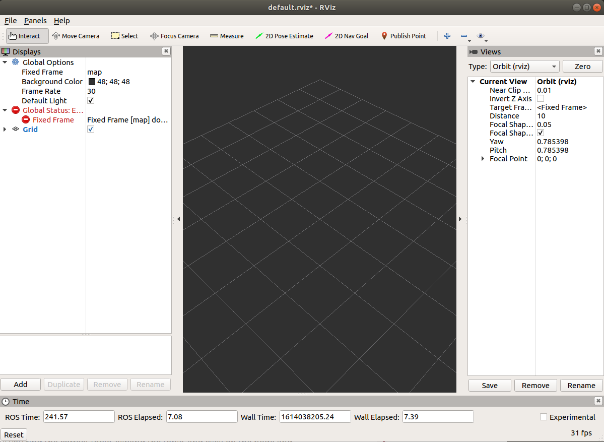
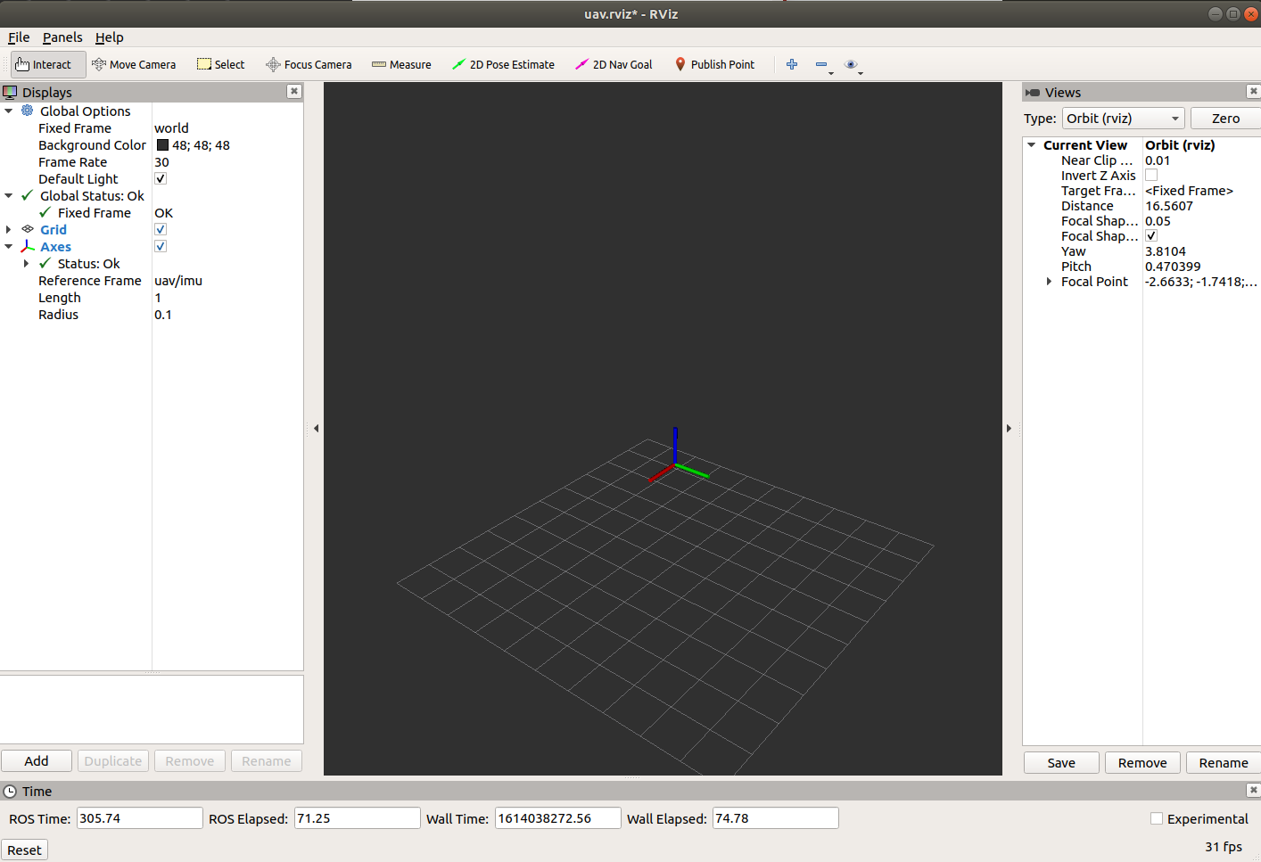
The screen is empty because RViz does not know what topics to listen to for our robot. RViz allows us to save configurations to disk. In the top left select “File” > “Open Config”. In the window that opens, navigate to /root/CS4501-Labs/lab4_ws/src/visualizer/rviz and select the saved configuration uav.rviz. You should now see a set of axes float around above the grid. That’s our robot! RViz has support for visualizing more complex robot models, but the robot axes positioned at the center of the robot will suffice for our goals.
Adding the LIDAR to RViz
Now that we can see our robot, we want to visualize the LIDAR data. In the lower left in RViz, click the “Add” button. The pop up gives us the option to either add “By display type” or “By topic”. Since we know the LIDAR topic, select “By topic”, scroll down until you find the correct topic, expand the topic, and click on the node and click OK. The LIDAR should appear as floating dots above the grid:
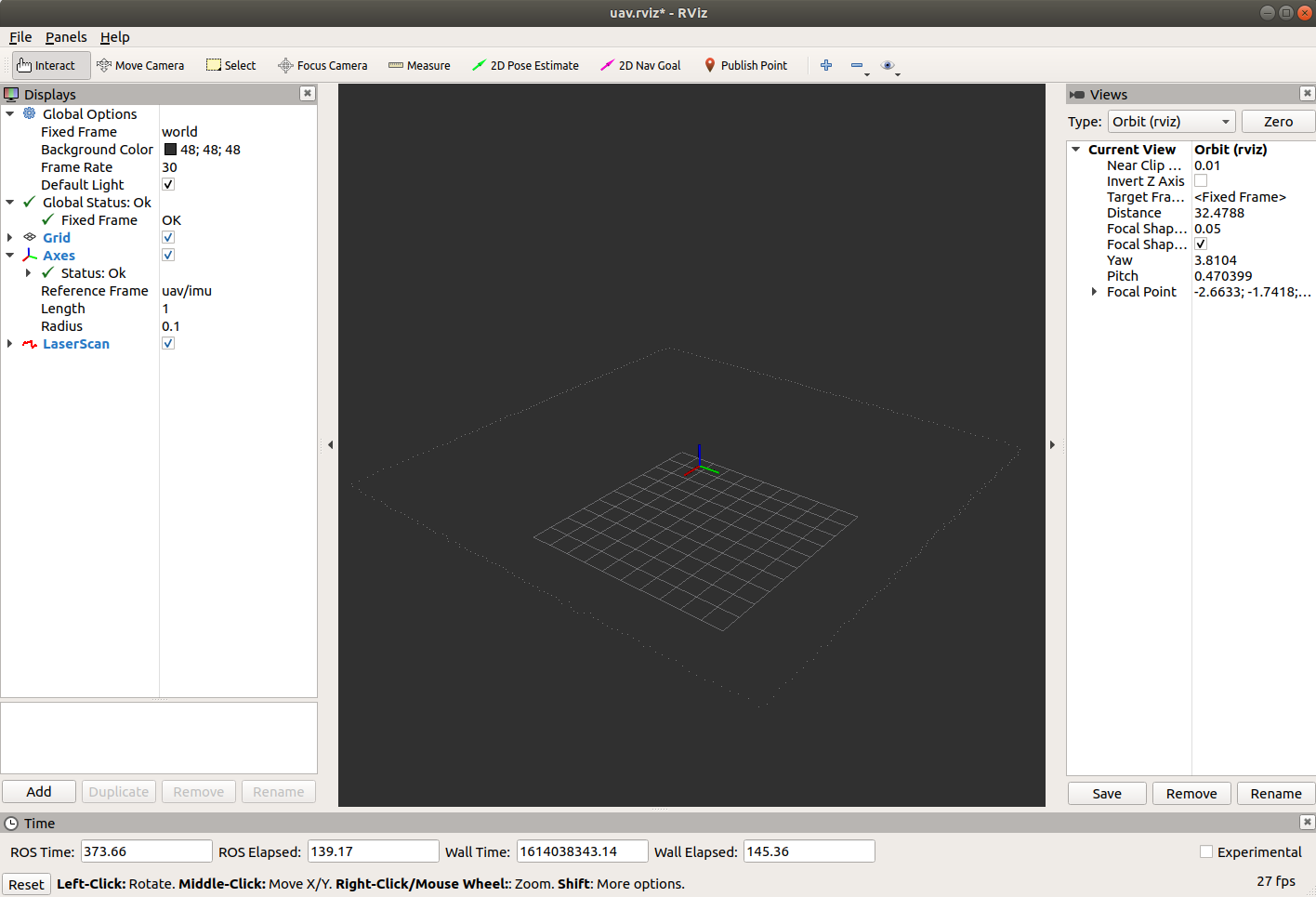
You will notice that there are gaps in the LIDAR. This is because RViz is displaying the points too small. On the left side, find the topic for the LIDAR, expand it and find the “Size (m)” entry. Click on the “0.01” and change it to “0.05”. If this does not make the points visible, find the “Style” entry and change “Flat Squares” to “Points” and then change size to 2.
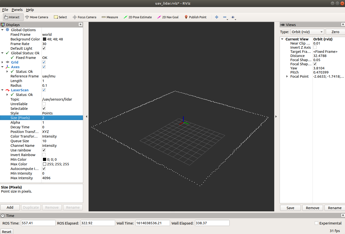
The visualization of the LIDAR data from the robot sensing the room.
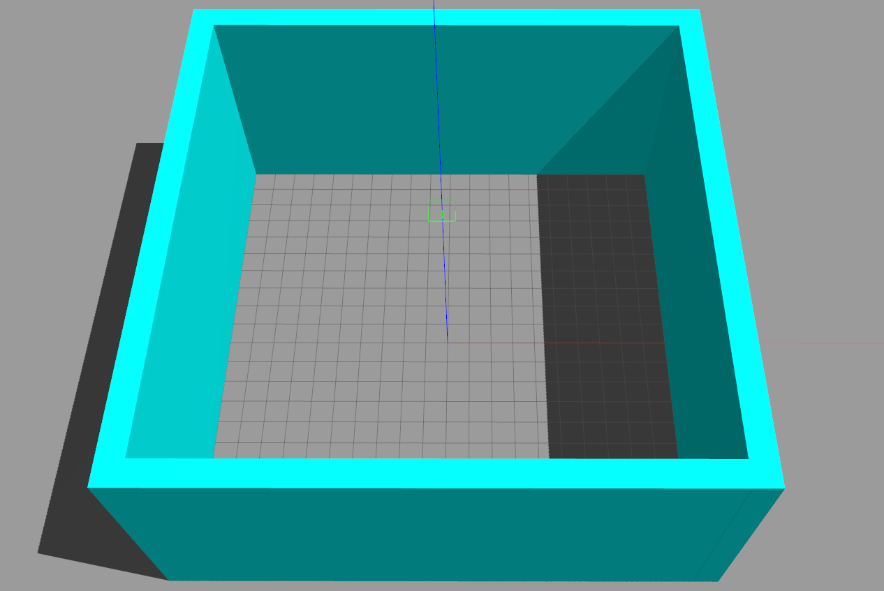
The physical environment the LIDAR is sensing.
We can now see all of the LIDAR points and get a better picture of the room we are in! Now we want to save the config for later so that we don’t have to perform this set up again. Select “File” > “Save Config As”. In the ~/CS4501-Labs/lab4_ws/src/visualizer/rviz directory, save this as uav_lidar.rviz. Close RViz and stop the simulator.
While the initial configuration in uav.rviz was provided with the lab, you are now equipped to set up RViz from scratch. Even for complicated projects, configuring RViz is a matter of adding the right topics and configuring the visualization to help the end-user understand what the robot is seeing. For more information on other available options, refer to the RViz User Guide.
Sensing a New Environment
Open the fly.launch file that we have been using. Because this is a simulator, we must tell the LIDAR what enviroment to simulate. You will see that the sensors node take as input the map file to do this. In this case, the map file is very simple and purpose-built for our lab; however, map files are very commonly used in simulation and there are many standard formats such as .sdf and .xodr used for different simulators.
  <include file="$(find sensor_simulation)/launch/sensors.launch">
    <arg name="map_path" value="room.txt" />
  </include>
Change room.txt to room2.txt. Relaunch the simulator.
Checkpoint 1
- Open RViz and load the
uav_lidar.rvizconfig. Take a screenshot ofroom2. - What shape is
room2?
Filtering and Combining Sensor Data
As we know, sensors are noisy. Every aspect of a robot’s actions require accurate knowledge of the physical world, and noise in the sensed measurements of the world can affect the robot’s ability to safely perform its tasks. In order for us to deal with that noise and get accurate sensor readings, we need some way to model and account for noise. In this lab, we will examine several methods of dealing with noise and reducing uncertainty. Each method will introduce a new level of complexity, but will result in a reduced level of uncertainty which in turn will improve performance.
To model noise and uncertainty in sensors, we can think of the value the sensor reports as a random variable. Typically, we model this as a Gaussian normal distribution (N(μ,σ)) with the sample mean centered on the actual value and the standard deviation being based on the sensor characteristics. In practice, when the robot reads the value from the sensor, it is sampling from this distribution with the goal of determining the actual value. Sometimes the uncertainty in the reading is low, or the robot only needs a rough estimate and so the value of the sensor can be used directly. However, if the sensor is very uncertain or noisy, or if the robot needs to know the precise value, then additional steps must be taken to generate a better value. We will examine using a simple moving average filter, sensor fusion, and a Kalman Filter to solve this problem.
We will study this in the context of the altitude of the robot. The altitude of the robot is provided as a z coordinate by the GPS sensor. Additionally, we will calculate the altitude using a LIDAR that is mounted toward the ground. We will begin by using a moving average filter on both the values provided by the GPS and the LIDAR altitude to smooth out the variance of the data. Then we will use sensor fusion to calculate an average of the two moving averages. Finally, we will examine how to use a Kalman Filter to estimate altitude.
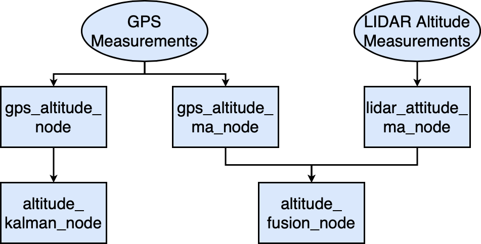
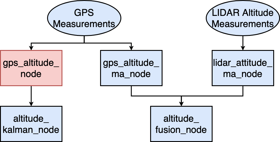
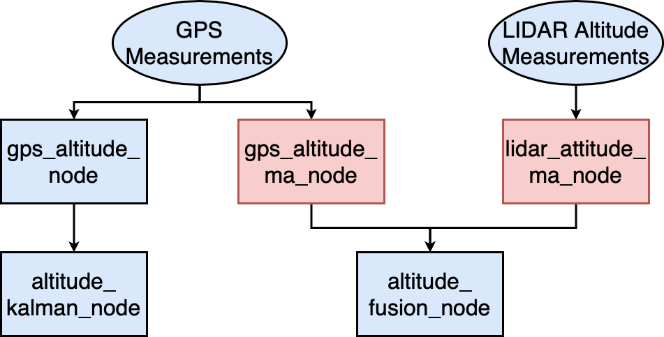
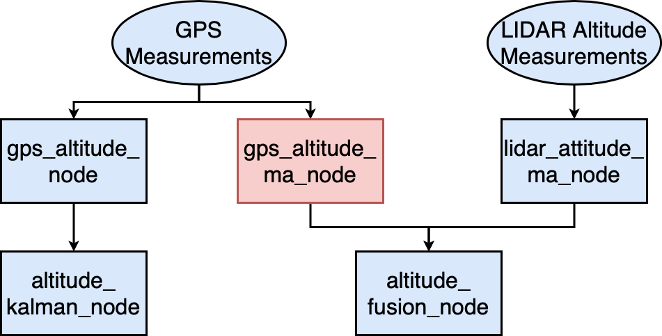
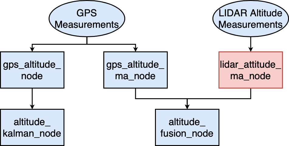
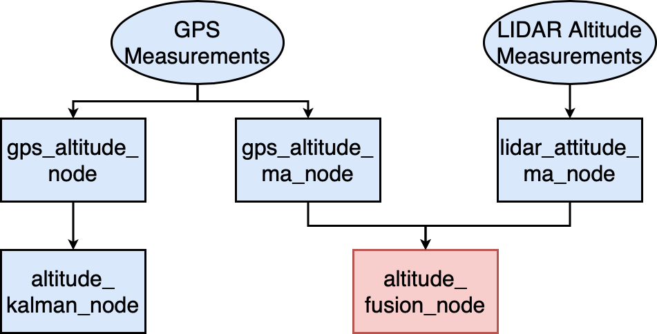
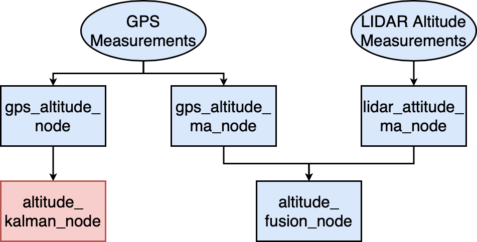
Architecture
This image serves as a roadmap for the nodes that we will implement throughout the lab. In the images below, ma stands for Moving Average, which we will explore as the first technique for noise reduction.
A Message Type for Altitude
We want to develop reusable code to handle sensor data that deals with altitude. In order to make our code modular and reusable in the future, we will create a new package that contains our nodes along with a custom message type to store altitude data.
Create the altitude package:
cd ~/CS4501-Labs/lab4_ws/src/
catkin_create_pkg altitude std_msgs geometry_msgs rospy message_generation message_runtime
Let’s begin by creating the custom message type for the altitude measurements. As we have discussed in previous labs, in general you should try to re-use built-in message types whenever possible. However, here we are going to model the error in the measurement and pass it as a part of the message, so we will use this opportunity to learn how to create a new message type. Creating a message is very similar to how we created services in the previous lab. We need to create the message definition file, which we call AltitudeStamped.msg, define what the message will contain and then configure the ROS workspace to build these messages.
cd ~/CS4501-Labs/lab4_ws/src/altitude
mkdir msg
touch msg/AltitudeStamped.msg
Now open AltitudeStamped.msg in your favorite editor and insert the following:
float64 value
float64 error
time stamp
This is the specification of your message type. The new message has type AltitudeStamped and contains three attributes: value of type float, error of type float, and stamp of type rospy.time. value will contain the altitude, error will contain the standard deviation of measurement for the altitude, and stamp will contain the time this measurement was taken.
Now that we have created the specification of the message in the AltitudeStamped.msg file, we need to update CMakeLists.txt and package.xml so that the message type will be processed. These two files tell catkin what to process when we run catkin build, so we need to tell them to build our new message type too. More information on using catkin with CMakeLists.txt and package.xml can be found on the ROS wiki.
Add the following lines in altitude/CMakeLists.txt if they are not already there. These tell CMakeLists.txt that we have a new message file that needs to be generated, and that we depend on the message_runtime package to do so. Add the following lines after the find_package block.
add_message_files(
  FILES
  AltitudeStamped.msg
)
generate_messages(
   DEPENDENCIES
   std_msgs
)
catkin_package(
  CATKIN_DEPENDS message_runtime
)
Then add the following line to altitude/package.xml. This indicates that our package depends on the message_runtime package in order to build.
<build_depend>message_runtime</build_depend>
To check that the message is created correctly, build the workspace, source it and run the command below:
rosmsg show altitude/AltitudeStamped
The expected output is the content of AltitudeStamped.msg,
float64 value
float64 error
time stamp
Using our Altitude Message
The RViz file that we used earlier uses the axes to show the actual position of the drone. We have access to the ground truth position because we are using a simulator and thus we can ask the simulator for the exact position of the robot. Normally, this will not be the case when the system is deployed, and we will have to rely on our sensors to determine the position. Let’s use our new AltitudeStamped message class to report the altitude of the robot as measured by the GPS.
Using GPS to send an Altitude Message
We will now add a node that takes the GPS position as input and publishes the altitude.
cd ~/CS4501-Labs/lab4_ws/src/altitude/src
touch gps_altitude.py
chmod u+x gps_altitude.py
Copy the following code into gps_altitude.py
#!/usr/bin/env python
import rospy
import time
from geometry_msgs.msg import PoseStamped
from altitude.msg import AltitudeStamped

class GPSAltitude:
    # Node initialization
    def __init__(self):
        # Create the publisher and subscriber
        self.pub = rospy.Publisher('/uav/sensors/altitude',
                                   AltitudeStamped,
                                   queue_size=1)
        self.sub = rospy.Subscriber('/uav/sensors/gps_noisy',
                                    PoseStamped, self.process_altitude,
                                    queue_size=1)
        self.gps_error = float(rospy.get_param('/uav/sensors/position_noise_lvl', str(0)))
        self.altitude = AltitudeStamped()
        self.gps_pose = PoseStamped()
        rospy.spin()

    def process_altitude(self, msg):
        self.gps_pose = msg
        self.altitude.value = self.gps_pose.pose.position.z
        self.altitude.stamp = self.gps_pose.header.stamp
        self.altitude.error = self.gps_error
        self.pub.publish(self.altitude)


if __name__ == '__main__':
    rospy.init_node('gps_altitude_node')
    try:
        GPSAltitude()
    except rospy.ROSInterruptException:
        pass
This code takes in the GPS reading and outputs an AltitudeStamped message. It uses ros_param to find out the error in the GPS sensor. Normally the GPS error would be something you find on the datasheet for the GPS module you are using. However, since this is a simulator the GPS error can be configured through ros_param and is usually chosen to mimic expected conditions, or is inflated to stress test the system. Add gps_altitude.py to the main launch file.
Visualizing the Altitude
As we learned with the altitude package, it is always a good idea to keep code modular and reusable. Our workspace contains lots of code for running a drone and each of the packages is responsible for a different part of the process. Think about what would need to happen for us to run on a real drone. We would need to have some way of translating the internal topics into commands that get sent to the real motors. This could be done with another package that we use depending on which type of real drone we use. Since we are working in simulation, we need to be able to see a simulated drone. This is what the visualizer package does. This package was provided with the lab and contains the code to run the plotting window we were using before RViz. Earlier in the lab, we saved the RViz config files in the visualizer package as well. Now, we will add a node to the visualizer package that publishes the altitude data in a format RViz can easily display. Run the following in a terminal to create the new node:
cd ~/CS4501-Labs/lab4_ws/src/visualizer/src
touch altitude_visualizer.py
chmod +x altitude_visualizer.py
Now, copy the following code into altitude_visualizer.py
#!/usr/bin/env python
import rospy
import time
from geometry_msgs.msg import PoseStamped
from altitude.msg import AltitudeStamped
from visualization_msgs.msg import Marker


class AltitudeVisualizer:
    # Node initialization
    def __init__(self):
        # Create the publisher and subscriber
        self.marker_pub = rospy.Publisher('/uav/visualizer/altitude_marker',
                                   Marker,
                                   queue_size=1)

        self.sub = rospy.Subscriber('/uav/sensors/altitude',
                                    AltitudeStamped, self.process_altitude,
                                    queue_size=1)

        self.sub = rospy.Subscriber('/uav/sensors/altitude_ma',
                                    AltitudeStamped, self.process_altitude_ma,
                                    queue_size=1)

        self.sub = rospy.Subscriber('/uav/sensors/altitude_fused_ma',
                                    AltitudeStamped, self.process_altitude_fused_ma,
                                    queue_size=1)

        self.sub = rospy.Subscriber('/uav/sensors/altitude_kalman',
                                    AltitudeStamped, self.process_altitude_kalman,
                                    queue_size=1)
        rospy.spin()

    def process_altitude(self, msg):
        self.generate_marker(msg, 0, (1, 1, 0))  # yellow

    def process_altitude_ma(self, msg):
        self.generate_marker(msg, 1, (0, 1, 0))  # green

    def process_altitude_fused_ma(self, msg):
        self.generate_marker(msg, 2, (1, 0, 0))  # red

    def process_altitude_kalman(self, msg):
        self.generate_marker(msg, 3, (1, 0, 1))  # magenta

    def generate_marker(self, msg, id, color):
        # the Marker message type is provided by RViz and contains
        # all of the fields that we need to set in order for it to
        # display our shapes.
        marker = Marker()
        # The frame_id string tells RViz what frame of reference to
        # use when drawing this Marker. In this case, the "imu_ground"
        # frame is generated by the provided lab code and has its
        # origin set on the xy-plane directly below the robot
        marker.header.frame_id = "uav/imu_ground"
        marker.header.stamp = msg.stamp
        marker.ns = "uav"
        # If you have multiple Markers, they each need a unique id.
        # Here, each of the different topics we are listening to
        # has its own id hard coded into the method call
        marker.id = id
        # RViz has several built in shapes, see the documentation
        marker.type = Marker.SPHERE
        marker.action = Marker.ADD
        # Below we set the location of the Marker. The "imu_ground"
        # reference frame has its origin directly below the robot,
        # so to have the Marker appear at the altitude of the robot,
        # we set the z position to be the altitude message value
        marker.pose.position.x = 0
        marker.pose.position.y = 0
        marker.pose.position.z = msg.value
        # Quaternions represent rotation. The below quaternion is
        # the "no rotation" quaternion. Since we have a sphere object
        # the rotation does not really matter.
        marker.pose.orientation.x = 0.0
        marker.pose.orientation.y = 0.0
        marker.pose.orientation.z = 0.0
        marker.pose.orientation.w = 1.0
        # This is the radius of the sphere. We want the size of the
        # sphere to represent the error in the measurement. The
        # larger the sphere, the less certain we are. If there are
        # multiple spheres, we can think of the volume of each sphere
        # as representing the 95% confidence interval for that value
        marker.scale.x = msg.error
        marker.scale.y = msg.error
        marker.scale.z = msg.error
        # The color is represented in (a,r,g,b). The alpha=0.5 tells
        # RViz to make the Marker semi-transparent. We do this so that
        # if two Markers intersect we can still see both. The color is
        # passed in as an argument to this function so that each topic
        # has its own color. You can refer above for the color mapping.
        marker.color.a = 0.5
        marker.color.r = color[0]
        marker.color.g = color[1]
        marker.color.b = color[2]
        self.marker_pub.publish(marker)


if __name__ == '__main__':
    rospy.init_node('altitude_visualization_node')
    try:
        AltitudeVisualizer()
    except rospy.ROSInterruptException:
        pass
This code uses the RViz display type Marker to send a message to display. We are using a sphere to represent the location of the robot. The center of the sphere represents the position and the radius of the sphere represents the error. The smaller the sphere, the less error there is in our measurement of position.
Add altitude_visualizer.py to the view.launch file in the visualizer package. Launch the simulator and open RViz. Load the uav_lidar.rviz config file from before. Using the same steps from above, add a visualization that listens to the topic /uav/visualizer/altitude_marker. Save the updated config to uav_altitude.rviz.
You should see something like the following:
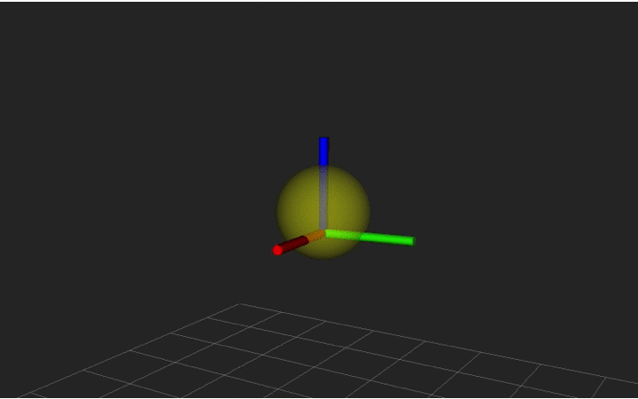
The yellow ball will be jumping up and down along the z-axis, though it should stay roughly centered around the actual location of the drone. This is because we are using a noisy sensor; each time we receive a position, we are sampling from a random distribution that is centered around the true altitude. The size of the ball corresponds to the amount of uncertainty in our measurement. In the next section we will look at ways to combat that noise.
Using a Moving Average Filter
One of the very common simple filters used for noisy data is a Moving Average Filter. You have probably seen a moving average filter used when reporting COVID-19 cases. For example, the Virginia Department of Health graphs the data showing both the number of cases each day and the 7-day moving average. They use a 7-day filter because the number of cases each day is biased depending on the day. For example, the number of tests performed/processed over the weekend is lower than that during the week, which leads to dips in the graph – but that doesn’t mean there are fewer cases on the weekend. Because of this, averaging over a week provides a clearer picture of the data trends.
Similarly, for robotics sensors, moving averages can help us get a clearer picture of the actual value underlying the noise. More generally, from statistics, we know that the more measurements we take from a distribution, the closer the mean of that population will be to the underlying distribution. Moving averages leverage that principle while allowing for the fact that we may be tracking a moving object; averaging over all time doesn’t make sense if the robot is moving, but we may be willing to take an average over a few steps to get less uncertainty even if the information is outdated.
Implementing Moving Average
We will implement two nodes that compute the moving average of altitude, one that uses the GPS sensor data and one that uses the LIDAR sensor data.
First, we will implement the code for computing the moving average into a Python package that can be imported in the ROS nodes (not depicted in the picture above).
cd ~/CS4501-Labs/lab4_ws/src/altitude/src
touch moving_average.py
Implement the MovingAverage class in the file named moving_average.py with the following signature and specification. You are welcome to implement the moving average class however you wish as long as it conforms to this specification. Note: This is not a ROS node. This is a class we will use in a different ROS node later.
# The MovingAverage implements the concept of window in a set of measurements.
# The window_size is the number of most recent measurements used in average.
# The measurements are continuously added using the method add.
# The get_average method must return the average of the last window_size measurements.
class MovingAverage:
    def __init__(self, window_size):
        #TODO
        pass

    # add a new measurement
    def add(self, val):
        #TODO
        pass

    # return the average of the last window_size measurements added
    # or the average of all measurements if less than window_size were provided
    # if no values have been added, return 0
    def get_average(self):
        #TODO
        pass
Hint: you may consider using the Python deque type to implement the underlying data structure in your moving average.
Testing Moving Average
The moving average code that we have written is general and it may be used by many clients. But before it is used by others, it is always a good software engineering practice to unit test our code to detect faults as early as possible before they affect other parts of the system. In this lab, we will take advantage of Python’s unit test framework to make our job easier.
cd ~/CS4501-Labs/lab4_ws/src/altitude/src
touch test_moving_average.py
Copy the below test code into test_moving_average.py
import unittest

from random import seed
from random import random

import numpy as np

from moving_average import MovingAverage


class TestMovingAverage(unittest.TestCase):

    def setUp(self):
        pass

    def test_empty_window(self):
        mw = MovingAverage(10)
        self.assertEqual(mw.get_average(), 0.0)

    def test_short_window(self):
        mw = MovingAverage(10)
        values = [random() for i in range(5)]
        for v in values:
            mw.add(v)
        self.assertTrue(abs(mw.get_average() - np.average(values) <= 0.0001))

    def test_window(self):
        mw = MovingAverage(5)
        values = [random() for i in range(10)]
        for v in values:
            mw.add(v)
        self.assertTrue(abs(mw.get_average() - np.average(values[5:]) <= 0.0001))

    def test_window_changing(self):
        mw = MovingAverage(5)
        zero_values = [random() for i in range(5)]
        for v in zero_values:
            mw.add(v)
        self.assertTrue(abs(mw.get_average() - np.average(zero_values) <= 0.0001))
        five_values = [5 + random() for i in range(5)]
        for v in five_values:
            mw.add(v)
        self.assertTrue(abs(mw.get_average() - np.average(five_values) <= 5.0001))
Run the test using the command below:
python -m unittest test_moving_average
>>> ----------------------------------------------------------------------
>>> Ran 4 tests in 0.000s
>>> OK
When testing it is important to think about what special cases your code needs to handle. Think about what cases the above tests exercise.
Moving Average for Altitude
Now that we have code that can compute moving averages for us, we will create a node that uses it to give us a more accurate position. We will use the existing gps_altitude.py node as a baseline, so begin by making a copy.
cd ~/CS4501-Labs/lab4_ws/src/altitude/src
cp gps_altitude.py gps_altitude_ma.py
You will also need to update the fly.launch file accordingly; include both gps_altitude.py and gps_altitude_ma.py in the launch file.
First, update the class name to GPSAltitudeMA. Then, update the __init__ to create a MovingAverage with a window size of 5. Also update the publisher to send to a new topic, /uav/sensors/altitude_ma.
from moving_average import MovingAverage
# ...
    # Node initialization
    def __init__(self):
        self.pub = rospy.Publisher('/uav/sensors/altitude_ma',
                                   AltitudeStamped,
                                   queue_size=1)
        self.moving_average = MovingAverage(5)
# ...
Then, in the process_altitude callback, use the message to update the moving average.
#...
    def process_altitude(self, msg):
        self.gps_pose = msg
        self.moving_average.add(self.gps_pose.pose.position.z)
        self.altitude.value = self.moving_average.get_average()
#...
The final step is to update the error. The propagation of uncertainty is a useful concept from statistics that allows us to reason about the uncertainty or error in our sensed values. We started with a single measurement that we knew had error self.gps_error. Now that we have aggregated 5 measurements, we expect that we will have a lower uncertainty in our measurement. The formula in this case (in pseudocode) is moving_average_error = original_error / sqrt(window_size).
Update the self.altitude.error field to the new value and relaunch the simulator and load the uav_altitude.rviz RViz config. You should see a new Marker for the moving average data. Note that it could overlap with the original Marker.
Checkpoint 2
- What cases do the unit tests in
test_moving_averag.pycover? - Take a screenshot of your RViz set up.
- How does the new ball compare in size to the old one? Why?
- How does the movement of the new ball compare to the old one? Why?
- How does changing the window size affect the error?
- What information do we lose by using moving average instead of individual measurements?
Sensor Fusion
Taking a moving average of our sensor data can help us reduce noise and improve our estimates. However, we have more information we can use to improve our GPS altitude estimate by combining it with other sensors. For example, in our system the LIDAR node senses its environment and, if it is given a map, it can determine and publish its estimated position to the topic /uav/sensors/lidar_position.
In practice, a LIDAR sensor provides a point cloud that requires additional processing to provide a position. This processing is usually provided by localization algorithms. ROS includes a few of such algorithms such as AMCL.
We will now create a LIDAR altitude moving average node using the GPS version as a model.
cd ~/CS4501-Labs/lab4_ws/src/altitude/src
cp gps_altitude_ma.py lidar_altitude_ma.py
Update the node lidar_altitude_ma to reflect the name change. You also need to update:
- Publish to the
/uav/sensors/lidar_altitude_matopic - Subscribe to the
/uav/sensors/lidar_positiontopic- Since this topic uses a different message type, you need to update both code subscriber definition and callback accordingly.
- The error should come from the
/uav/sensors/lidar_position_noiseparameter.
Add this node to fly.launch.
Next we will add a node that fuses together the altitude values from both sensors. Create the file altitude_fusion.py:
cd ~/CS4501-Labs/lab4_ws/src/altitude/src
touch altitude_fusion.py
chmod u+x altitude_fusion.py
Using your favorite editor, start with the following code as a baseline:
#!/usr/bin/env python
import rospy
import time
from threading import Lock
from altitude.msg import AltitudeStamped
class AltitudeFusion:

    # Node initialization
    def __init__(self):
        self.lidar_altitude = 0
        self.lidar_error = 0
        self.gps_altitude = 0
        self.gps_error = 0
        self.last_timestamp = None
        self.changed = False
        self.lock = Lock()
        # Create the publisher and subscriber
        self.pub = rospy.Publisher('/uav/sensors/altitude_fused_ma',
                                   AltitudeStamped,
                                   queue_size=1)
        self.la_sub = rospy.Subscriber('/uav/sensors/lidar_altitude_ma',
                                 AltitudeStamped, self.process_lidar_altitude,
                                    queue_size = 1)
        self.pa_sub = rospy.Subscriber('/uav/sensors/altitude_ma',
                                  AltitudeStamped, self.process_gps_altitude,
                                    queue_size = 1)
        self.mainloop()

    def process_lidar_altitude(self, msg):
        self.lock.acquire()
        #TODO
        self.changed = True
        self.lock.release()
    def process_gps_altitude(self, msg):
        self.lock.acquire()
        #TODO
        self.changed = True
        self.lock.release()


    # The main loop of the function
    def mainloop(self):
        # Set the rate of this loop
        rate = rospy.Rate(10)
        # While ROS is still running
        while not rospy.is_shutdown():
            avg_msg = None
            self.lock.acquire()
            if self.changed and self.lidar_error > 0 and self.gps_error > 0:
                #TODO initialize avg_msg
                self.changed = False
            self.lock.release()
            if avg_msg:
                self.pub.publish(avg_msg)
            # Sleep for the remainder of the loop
            rate.sleep()

if __name__ == '__main__':
    rospy.init_node('altitude_fusion_node')
    try:
        AltitudeFusion()
    except rospy.ROSInterruptException:
        pass
You need to implement the following:
- In
process_lidar_altitudeupdateself.lidar_altitudeandself.lidar_errorusing the value from the message - In
process_gps_altitudeupdateself.gps_altitudeandself.gps_errorusing the value from the message - In each of the callbacks, update
self.last_timestamp - In
mainloopcreate a new message of typeAltitudeStampedwith the last time stamp received as stamp. Set the mean and error as described below.
Propagation of Error in Sensor Fusion
Recall from before that we can model each sensor as a random variable, namely a Gaussian normal distribution with mean μ and standard deviation σ. When we combine the two distributions, they form a single distribution with a mean between the two original distributions and with a standard deviation lower than each of the originals:
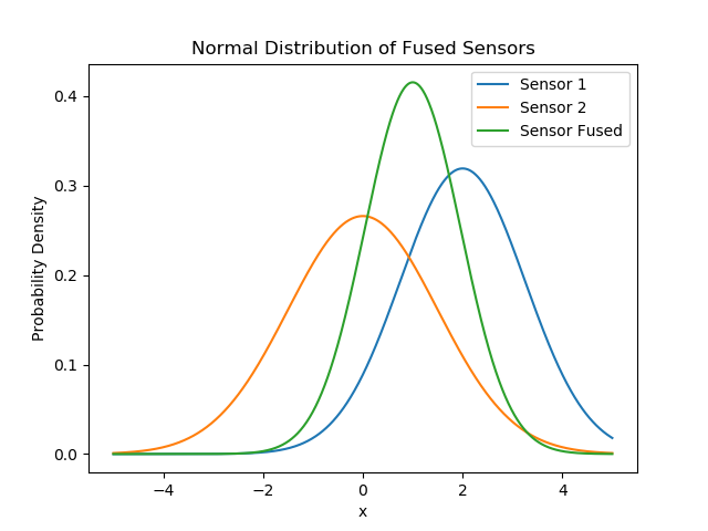
If sensor 1 has a mean of μ1 and standard deviation (error) σ1, and sensor 2 has a mean of μ2 and standard deviation σ2, then the distribution of the fused sensor has mean and standard deviation:
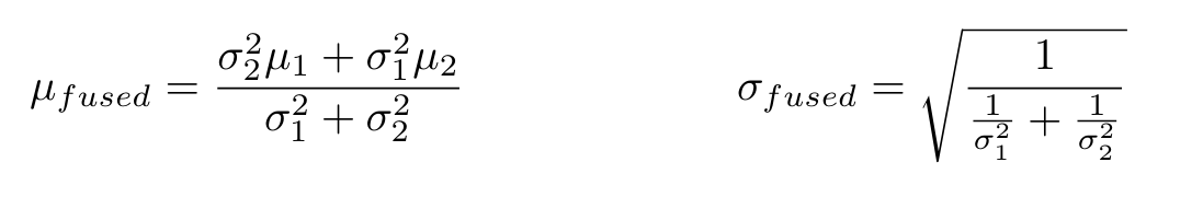
Use these formulae to implement the error in the AltitudeStamped message, with the sensor measurement in place of the mean and σfused for the error.
Locking and Threads
In the code for the GPS and LIDAR moving average nodes, the message received in the callback was processed and the corresponding message published on one single thread, so no synchronization was necessary. In the code above, however, there are three threads: one for each subscriber and one for the mainloop. Furthermore, the three threads share variables for the altitudes, errors, and the last timestamp. Without proper synchronization, we could get some strange behaviors like having an updated value of one of the variables containing the altitude with an old timestamp.
We use a lock to help synchronize the threads and prevent such race conditions (the lock is an instance of the type threading.Lock). The code ensures that only one thread may hold the lock at a time. If the lock is available then the acquire method returns immediately and the lock is allocated to the thread on which the acquire method was called. The lock is released when the release method is called from the same thread. If the lock is held by a thread A and another thread B calls to try to acquire the same lock, then thread B is blocked in the call and will wait until the lock is released. If thread A never releases the lock, then the thread B is blocked at the acquire call indefinitely. Locking can also help us to deal with situations where two threads need to share the same physical resource For example, if thread A and thread B both need to print a document, we can use locks to make sure that only one of them can communicate with the printer at a time.
Viewing the Fused Sensor Data
Add altitude_fusion.py to fly.launch. Launch the simulation and load RViz using the uav_altitude.rviz configuration.
Checkpoint 3
- Take a screenshot of your RViz set up.
- How does the new ball compare in size to both the one from the moving average and the original? Why?
- How does the movement of the new ball compare to both of the others? Why?
- Which technique produced the most accurate reading?
Kalman Filters
Thus far we have explored moving averages and sensor fusion in order to improve our estimates of the robot’s position in the real world. However, these methods have their drawbacks. For moving averages, we have to store several previous measurements to use in the average. Depending on the situation, the measurement received in the past may not be relevant to the current measurement, and thus the average could be of little use. Consider if the robot was in the process of gaining altitude - that motion would make our moving average data outdated. Sensor fusion improves on this, but is still limited in how far we can decrease our error without buying more or better sensors which can be costly. If we need more certainty in our location, especially while moving, we need more advanced techniques.
The Kalman Filter addresses both of these shortcomings of sensor fusion. Kalman Filters maintain an internal state of what the last value was, and uses this to inform the current estimate. If the robot is sitting still, then the more measurements we take, the more sure we can be of its position. However, the Kalman Filter is also robust in helping us predict our position while the robot is moving. By using the velocity of the robot, the Kalman Filter can predict where to where the robot will be in the future. Then when a new position measurement comes in, it can compare that with the predicted value and increase its certainty. This feedback loop allows the robot to create much more certain estimates of its position than using measurements alone while also being able to predict its location in the future. Instead of only being able to fuse two sensors that provide altitude data, we can also use other type of sensor data, such as those that provide velocity data to inform our estimate. Kalman Filters work in two steps as shown below
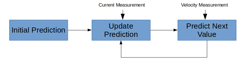
In our context, we begin with an initial prediction for our altitude in the form of a normal distribution with mean μi and standard deviation σi. We can either use our first sensor reading to initialize our prediction, or we can initialize our estimate to be very conservative. For example, we could say we think the drone’s position is described by a normal distribution with mean 0 and standard deviation of 100 to indicate that we think it is less than 100 units from the ground, but we are not sure where.
In the update step we take our current prediction for our estimate and combine that with our most recent sensor data using the same set of formulae discussed in the sensor fusion section. This gives us a newly updated prediction based on our last measurement that has a lower standard deviation than both our previous prediction and the measurement.
Once we have the updated prediction, we want to use the velocity measurement to create a new prediction. Since we are working with altitude, we only take the velocity in the z-axis. Our prediction is in units of altitude and the velocity is measured in units of altitude per time. Thus, we need to transform that velocity data into altitude as per distance = velocity * time. We then add that amount to our current position to obtain our new estimate for where we will be. The formulae for these steps are outlined below.
TREY: TODO: the equation on the feedback loop should be sigma_p
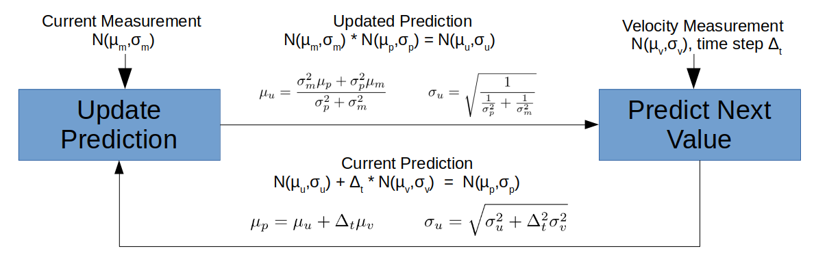
See this book for more information on Kalman Filters. The equations for Kalman Filters are very general, and we are only exploring the case of Gaussian normal variables in one dimension.
We will add a node that uses such a Kalman Filter to calculate a better altitude estimate. Create the file altitude_kalman.py:
cd ~/CS4501-Labs/lab4_ws/src/altitude/src
touch altitude_kalman.py
chmod u+x altitude_kalman.py
Using your favorite editor, start with the following code as a baseline:
#!/usr/bin/env python
import math

import rospy
from threading import Lock
from geometry_msgs.msg import TwistStamped
from altitude.msg import AltitudeStamped


class AltitudeKalman:

    # Node initialization
    def __init__(self):
        self.altitude = 0
        self.altitude_error = 0
        self.last_update = rospy.Time()
        self.velocity = 0
        self.lock = Lock()
        self.changed = False
        self.has_velocity_data = False
        self.predicted_altitude = None
        self.predicted_altitude_error = None
        self.velocity_error = float(rospy.get_param('/uav/sensors/velocity_noise_lvl', str(0)))
        # Create the publisher and subscriber
        self.pub = rospy.Publisher('/uav/sensors/altitude_kalman',
                                   AltitudeStamped,
                                   queue_size=1)
        self.altitude_sub = rospy.Subscriber('/uav/sensors/altitude',
                                    AltitudeStamped, self.process_altitude,
                                    queue_size=1)
        self.vel_sub = rospy.Subscriber('/uav/sensors/velocity_noisy',
                                       TwistStamped, self.process_velocity,
                                       queue_size=1)
        self.mainloop()

    def process_altitude(self, msg):
        self.lock.acquire()
        # TODO update data
        self.changed = True
        self.lock.release()


    def process_velocity(self, msg):
        self.lock.acquire()
        # TODO update velocity data, only using the z-axis
        self.has_velocity_data = True
        self.lock.release()

    # The main loop of the function
    def mainloop(self):
        # Set the rate of this loop
        rate = rospy.Rate(10)
        # While ROS is still running
        while not rospy.is_shutdown():
            self.lock.acquire()
            if self.changed and self.altitude_error > 0:
                if self.predicted_altitude is None:
                    self.predicted_altitude = self.altitude
                    self.predicted_altitude_error = self.altitude_error
                else:
                    # TODO use the altitude data to update the previous prediction
                    # Use the equations from the "Updated Prediction" part of the diagram above
                    pass
                self.changed = False
            if self.predicted_altitude is not None:
               if self.has_velocity_data:
                   current_time = rospy.Time.now()
                   delta_t = (current_time - self.last_update).to_sec() if self.last_update.to_sec() > 0 else 0
                   self.last_update = current_time
                   # TODO use the velocity data and the time since last update to create the current prediction
                   # Use the equations from the "Current Prediction" part of the diagram above
               kalman_msg = AltitudeStamped()
               # TODO fill in the altitude message based on the current predicted altitude and error
               self.pub.publish(kalman_msg)
            # Sleep for the remainder of the loop
            self.lock.release()
            rate.sleep()


if __name__ == '__main__':
    rospy.init_node('altitude_kalman_node')
    try:
        AltitudeKalman()
    except rospy.ROSInterruptException:
        pass
Add altitude_kalman.py to fly.launch. Launch the simulation and load RViz using the uav_altitude.rviz configuration.
Checkpoint 4
- Take a screenshot of your RViz set up. The Kalman Filter estimate is represented by a magenta ball. You may have to zoom in to see it.
- Use
rqt_plotto plot the following topics and take a screenshot of the plot:/uav/sensors/gps_noisy/pose/position/z/uav/sensors/gps/pose/position/z/uav/sensors/altitude_kalman/valueHow does the Kalman value compare with the other two topics? Which is it closer to?
Congratulations, you are done with Lab 4!
Final Check:
- Show the screenshot of RViz looking at
room2from checkpoint 1.- What shape is
room2?
- What shape is
- Show the screenshot of the RViz set up for checkpoint 2.
- What cases do the unit tests in
test_moving_averag.pycover? - How does the new ball compare in size with the old one? Why?
- How does the movement of the new ball compare with the old one? Why?
- How does changing the window size affect the error?
- What information do we lose by using moving average instead of individual measurements?
- What cases do the unit tests in
- Show the screenshot of the RViz set up for checkpoint 3.
- How does the new ball compare in size to both the moving average one and the original? Why?
- How does the movement of the new ball compare to both of the others? Why?
- Which technique produced the most accurate reading?
- Show the screenshot of the RViz set up for checkpoint 4.
- Show the screenshot of the
rqt_plot - How does the Kalman Filter value compare with the other two topics? Which is it closer to?
- Show the screenshot of the